Western diet drives gut resistome expansion in mice: a shotgun metagenomics analysis

1 Introduction

1.1 Background

• This report documents the replication of the shotgun metagenomics arm of Keskey et al. 2025
• The study tests whether a Western Diet (WD) — characterised by high fat (60% kcal) and absence of dietary fibre — independently increases the gut resistome (the collection of antibiotic resistance genes) in mice compared to a Standard Diet (SD) (18% kcal fat, 18 g fibre), without antibiotic exposure
• The dataset (PRJNA1148150) comprises 24 paired-end shotgun metagenomics samples from male C57BL/6 mice across three sample types: cecum (day 49 end-point), stool day 0 (baseline before diet intervention), and stool day 49 (end-point after 49 days of diet)
• Antibiotic resistance genes (ARGs) were detected via de novo assembly and screening against the Comprehensive Antibiotic Resistance Database (CARD) using Abricate, enabling both quantification of the gut resistome and linkage of ARGs to their bacterial host taxa via metagenome-assembled genomes (MAGs)

1.2 Rationale

• Replicating this analysis on publicly deposited data validates the original findings, documents a fully reproducible pipeline, and extends the ARG–taxon linkage using current Genome Taxonomy Database (GTDB) r226 taxonomy
• Using GTDB-Tk r226 for MAG taxonomy provides finer-grained species resolution and reflects current reclassification of the Bacteroides genus (including Phocaeicola spp.)

1.3 Materials

• ◼ WD (N = 12): 6 cecum, 3 stool day 0, 3 stool day 49
• ◼ SD (N = 12): 4 cecum, 4 stool day 0, 4 stool day 49
• Sample ID format: {group}_{animal}_{type} — three fields separated by underscores
  • group: diet assignment: SD (Standard Diet) or WD (Western Diet)
  • animal: zero-padded animal number (e.g. 01, 15, 26)
  • type: sample type and timepoint:
    • C: cecum, collected post-mortem at day 49
    • S0: stool, collected non-invasively at day 0 (baseline, before diet intervention)
    • S49: stool, collected non-invasively at day 49 (end-point, after 7 weeks on diet)
  • Example: SD_15_S49 — Standard Diet, animal 15, stool at day 49
• Sequencing: Illumina NovaSeq 6000 (150 bp paired-end), whole-genome shotgun; deposited by Cleveland Clinic
  • Four samples (SD_15_S49, SD_16_S49, WD_13_S0, WD_14_S0) were split across two SRA runs each and were concatenated prior to host removal

1.4 Computational methods

• Sequencing data preprocessing and host read removal
  1. SRA reads downloaded with prefetch + fasterq-dump
  2. Mouse host reads removed with Bowtie2 (--very-sensitive) against GRCm38; only concordantly unmapped read pairs retained
  3. Adapter trimming, quality filtering (Phred ≥ 20, length ≥ 50 bp), and PCR deduplication with fastp
  4. Per-sample reports aggregated with MultiQC
• Taxonomic classification
  1. Reads classified with Kraken2 (k2_standard database, confidence 0.1)
  2. Species-level abundance re-estimated with Bracken (read length 150 bp)
  3. Read attrition tracked at every step with a custom bash read-tracking script
• ARG detection and MAG taxonomy
  1. De novo assembly with MEGAHIT (--min-contig-len 200); contigs < 500 bp discarded
  2. ARG screening with Abricate v12 against CARD (--minid 80 --mincov 90, matching Keskey et al. 2025); hits with alignment length < 100 bp discarded
  3. Read-to-contig depth computed with Bowtie2 + jgi_summarize_bam_contig_depths
  4. Metagenomic binning with MetaBAT2; bin taxonomy assigned with GTDB-Tk r226
• Downstream analysis
  1. Species count matrix from Bracken; quality metrics from fastp/Bowtie2 logs
  2. Alpha diversity (rarefied) and beta diversity (Bray-Curtis PCoA + PERMANOVA) with vegan
  3. Taxonomic differential abundance with ANCOM-BC2 (Holm-Bonferroni correction)
  4. ARG proportion matrix (contigs carrying each ARG / total assembled contigs × 100)
  5. ARG differential abundance with White’s non-parametric t-test (BH FDR correction)
  6. ARG–taxon linkage via contig → MAG → GTDB-Tk species chain

2 Prerequisite

2.1 Environment

• OS: macOS 26.3.1
• Platform: aarch64-apple-darwin20
• Software: R (v4.5.1)
• Packages: ANCOMBC (v2.10.1), SummarizedExperiment (v1.38.1), TreeSummarizedExperiment (v2.16.0), coin (v1.4.3), dplyr (v1.1.4), ggplot2 (v4.0.1), ggrepel (v0.9.6), jsonlite (v2.0.0), plotly (v4.11.0), purrr (v1.1.0), readr (v2.1.5), scales (v1.4.0), tibble (v3.3.0), tidyr (v1.3.1), vegan (v2.7.2)

2.2 Computational workflow

• Bowtie2 — short-read aligner used for host read removal (GRCm38) and read-to-contig depth mapping
• Samtools — BAM/SAM processing; used with -f 12 -F 256 to extract both-unmapped read pairs
• fastp — adapter trimming, quality filtering (Phred ≥ 20, length ≥ 50 bp), and PCR deduplication
• MultiQC — aggregates per-sample fastp JSON reports into a single interactive QC summary
• Kraken2 — k-mer based taxonomic classification against the k2_standard database (93 GB)
• Bracken — probabilistic re-estimation of species-level abundances from Kraken2 reports
• MEGAHIT — de novo metagenome assembler; minimum contig length 200 bp at assembly, 500 bp after filtering
• Abricate v12 — screens contigs against CARD for ARGs; --minid 80 --mincov 90
• MetaBAT2 — bins assembled contigs into metagenome-assembled genomes using depth and tetranucleotide frequency
• GTDB-Tk r226 — assigns taxonomy to MAGs against the Genome Taxonomy Database release 226

2.3 Data acquisition

• SRA Toolkit: downloads paired-end FASTQs from NCBI SRA (PRJNA1148150) for all 24 SD and WD samples

#!/bin/bash

BASE_DIR="WORKING_DIRECTORY"
FASTQ_DIR="$BASE_DIR/fastq"
mkdir -p "$FASTQ_DIR"

# Example for a single accession; repeat for all SRR IDs
SRR="SRR12345678"
prefetch "$SRR" --output-directory "$FASTQ_DIR"
fasterq-dump "$FASTQ_DIR/${SRR}/${SRR}.sra" \
        --split-files \
        --outdir "$FASTQ_DIR" \
        --temp "$FASTQ_DIR" \
        --threads 8
gzip "$FASTQ_DIR/${SRR}_1.fastq" "$FASTQ_DIR/${SRR}_2.fastq"

2.4 Host read removal

• Bowtie2 + fastp + MultiQC: aligns reads to GRCm38 to remove mouse host reads, trims adapters, filters by quality (Phred ≥ 20, length ≥ 50 bp), removes PCR duplicates, and aggregates per-sample QC metrics

#!/usr/bin/env bash
# The following script is a template that was used to parallelize jobs in an HPC environment

bowtie2 -x "$BT2_INDEX" \
        -1 "$SCRATCH/${SAMPLE_ID}_R1.fastq.gz" \
        -2 "$SCRATCH/${SAMPLE_ID}_R2.fastq.gz" \
        --very-sensitive -p "$THREADS" \
        2> "$BASE_DIR/logs/host_rm/${SAMPLE_ID}_bt2.log" \
        | samtools view -f 12 -F 256 -b \
        | samtools sort -n -@ 4 -T "$SCRATCH/${SAMPLE_ID}" \
        | samtools fastq \
                -1 "$BASE_DIR/host_rm/${SAMPLE_ID}_R1.fastq.gz" \
                -2 "$BASE_DIR/host_rm/${SAMPLE_ID}_R2.fastq.gz" \
                -0 /dev/null -s /dev/null -@ 4

2.5 Taxonomic classification

• Kraken2 + Bracken: classifies microbial reads against the k2_standard database and re-estimates species-level abundances using a probabilistic redistribution model

#!/usr/bin/env bash
# The following script is a template that was used to parallelize jobs in an HPC environment

kraken2 \
        --db "$DB" \
        --paired --gzip-compressed \
        --threads "$THREADS" \
        --confidence 0.1 \
        --output "$BASE_DIR/kraken2/${SAMPLE_ID}.kraken2" \
        --report  "$BASE_DIR/kraken2/${SAMPLE_ID}.kreport" \
        --report-minimizer-data \
        "$BASE_DIR/trimmed/${SAMPLE_ID}_R1.fastq.gz" \
        "$BASE_DIR/trimmed/${SAMPLE_ID}_R2.fastq.gz" \
        2> "$BASE_DIR/logs/kraken2/${SAMPLE_ID}.log"

bracken \
        -d "$DB" \
        -i "$BASE_DIR/kraken2/${SAMPLE_ID}.kreport" \
        -o "$BASE_DIR/bracken/${SAMPLE_ID}.bracken" \
        -r 150 \
        -l S \
        -t 10

2.6 Metagenomic assembly

• MEGAHIT + MetaBAT2 + GTDB-Tk r226: assembles trimmed reads de novo into contigs; bins contigs into metagenome-assembled genomes (MAGs) using depth profiles and tetranucleotide frequency; assigns species-level taxonomy to each MAG against the Genome Taxonomy Database release 226

#!/usr/bin/env bash
# The following script is a template that was used to parallelize jobs in an HPC environment

# Step 1: Assembly
megahit \
        -1 "$BASE_DIR/trimmed/${SAMPLE_ID}_R1.fastq.gz" \
        -2 "$BASE_DIR/trimmed/${SAMPLE_ID}_R2.fastq.gz" \
        --out-dir "$SCRATCH/${SAMPLE_ID}_megahit" \
        --out-prefix "$SAMPLE_ID" \
        --min-contig-len 200 \
        --num-cpu-threads "$THREADS" \
        --memory 0.85
mkdir -p "$BASE_DIR/assembly/${SAMPLE_ID}"
cp "$SCRATCH/${SAMPLE_ID}_megahit/${SAMPLE_ID}.contigs.fa" \
        "$BASE_DIR/assembly/${SAMPLE_ID}/final.contigs.fa"

# Step 2: Filter contigs >= 500 bp
awk '/^>/ { if (seq != "" && length(seq) >= 500) print header"\n"seq;
             header = $0; seq = ""; next }
     { seq = seq $0 }
     END { if (seq != "" && length(seq) >= 500) print header"\n"seq }' \
        "$BASE_DIR/assembly/${SAMPLE_ID}/final.contigs.fa" \
        > "$BASE_DIR/assembly/${SAMPLE_ID}/contigs_500bp.fa"

2.7 ARG detection

• Abricate v12 (CARD): screens assembled contigs against the Comprehensive Antibiotic Resistance Database (CARD) for antibiotic resistance genes (ARGs); parameters match Keskey et al. 2025 (--minid 80 --mincov 90); hits with alignment length < 100 bp discarded

#!/usr/bin/env bash
# The following script is a template that was used to parallelize jobs in an HPC environment

# Step 3: ARG detection (Abricate v12 against CARD)
abricate \
        --db card \
        --minid 80 \
        --mincov 90 \
        --threads "$THREADS" \
        "$BASE_DIR/assembly/${SAMPLE_ID}/contigs_500bp.fa" \
        > "$BASE_DIR/abricate/${SAMPLE_ID}.tsv"

2.8 Preparation in the R environment

# Do not run — set this to your local project folder before re-running
base_dir <- "WORKING_DIRECTORY"
setwd(base_dir)

2.9 Load packages

library(ANCOMBC)
library(coin)
library(dplyr)
library(ggplot2)
library(ggrepel)
library(jsonlite)
library(plotly)
library(purrr)
library(readr)
library(scales)
library(tibble)
library(tidyr)
library(TreeSummarizedExperiment)
library(vegan)

2.10 Helper functions

• User-defined functions that can be reused throughout the analysis.

format_pval <- function(p) {
        if (is.na(p)) return("p = NA")
        if (p < 0.001) return("p < 0.001")
        paste0("p = ", formatC(p, format = "f", digits = 3))
}

theme_hub <- function(base_size = 11) {
        theme_bw(base_size = base_size) +
        theme(
                panel.grid.major = element_blank(),
                panel.grid.minor = element_blank(),
                strip.background = element_rect(fill = "grey95", colour = NA),
                strip.text       = element_text(face = "bold")
        )
}

3 FASTQ quality control

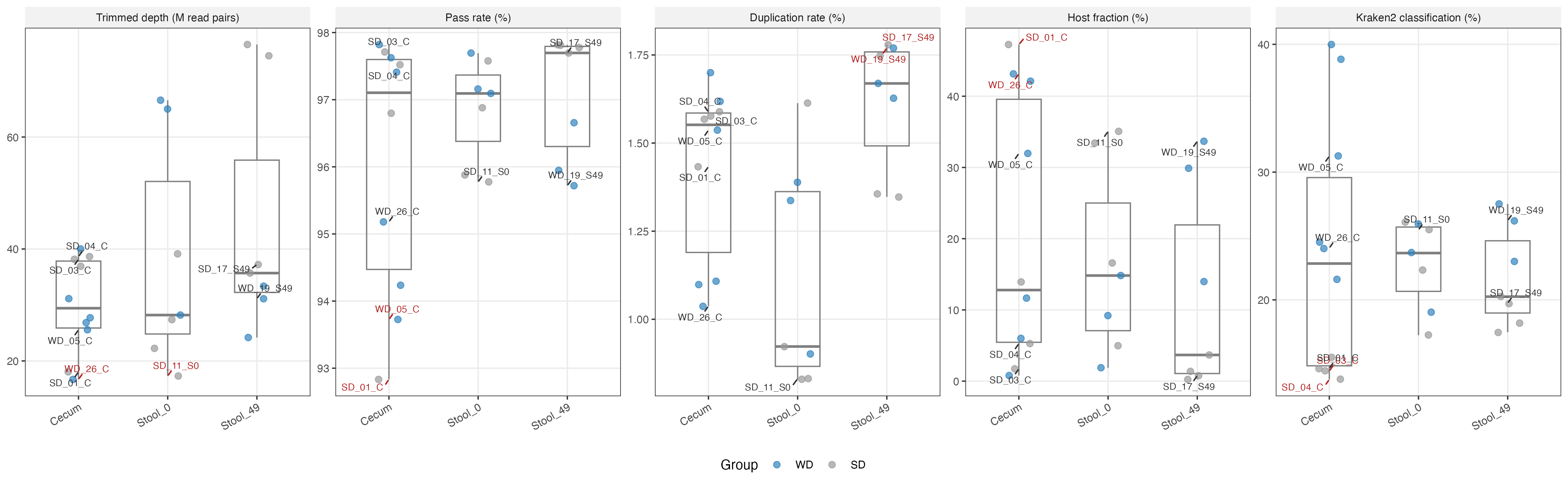
Summary: All 24 samples passed per-sample fastp processing. Two samples — SD_01_C (host fraction > P95) and WD_26_C (trimmed depth < P5) — were flagged as QC outliers and excluded from differential abundance analyses. All other samples were retained.

• Overall FASTQ quality (MultiQC) and Per-sample fastp QC reports
• QC metrics (trimmed depth, pass rate, duplication rate, host fraction, Kraken2 classification rate) visualised as strip charts stratified by sample type and diet group
  • WD_26_C was excluded due to low sequencing depth after host read removal and quality trimming, falling below the threshold required for diversity and differential abundance analyses
  • SD_01_C was excluded due to an abnormally high host (mouse) read fraction, indicating the sample was dominated by GRCm38-mapping reads rather than microbial reads, leaving insufficient metagenomic depth for reliable community profiling

qc <- readRDS(file.path(base_dir, "data", "qc_metrics.rds"))

head(qc)

## # A tibble: 6 × 14
##   sample_id group sample_type trimmed_depth_pairs pass_rate_pct dup_rate_pct
##   <chr>     <fct> <fct>                     <dbl>         <dbl>        <dbl>
## 1 SD_01_C   SD    Cecum                  18050994          92.8        1.43 
## 2 SD_02_C   SD    Cecum                  36899802          96.8        1.58 
## 3 SD_03_C   SD    Cecum                  38152851          97.7        1.57 
## 4 SD_04_C   SD    Cecum                  38642357          97.5        1.59 
## 5 SD_08_S0  SD    Stool_0                39128630          97.6        1.61 
## 6 SD_09_S0  SD    Stool_0                27373568          96.9        0.829
## # ℹ 8 more variables: host_frac_pct <dbl>, kraken2_rate_pct <dbl>,
## #   flag_depth <lgl>, flag_pass <lgl>, flag_dup <lgl>, flag_host <lgl>,
## #   flag_kraken <lgl>, flagged <lgl>

4 Analysis

4.1 Species count matrix

Summary: Bracken output from 24 samples (28 files including multi-run pairs) was merged into a species × sample count matrix of estimated read counts at the species level.

• Per-sample Bracken .bracken files parsed and read counts aggregated; multi-run samples (SD_15_S49, SD_16_S49, WD_13_S0, WD_14_S0) summed across runs per taxon before matrix construction
• Counts represent Bracken-estimated read counts, not raw read fractions
• The matrix is used directly by diversity and differential abundance analyses

bc <- readRDS(file.path(base_dir, "data", "bracken_counts.rds"))
counts_mat <- bc$counts
meta       <- bc$metadata

head(counts_mat[, 1:5])

##                              SD_01_C SD_02_C SD_03_C SD_04_C SD_08_S0
## Treponema phagedenis              26      64      37       0       43
## Campylobacter jejuni            4041     491    4113     493        0
## Proteus mirabilis               1478     397       0       0     1705
## Bacteroides fragilis            4540   16826   12597   14905    10652
## Bacteroides thetaiotaomicron   21245   28437   16924   17357    30483
## Bacteroides uniformis          66122  131599  174168  169067   175557

4.2 Microbial community diversity

Summary: WD mice showed significantly lower alpha diversity and near-complete community separation from SD mice along the first beta diversity axis. The reduction was driven primarily by loss of evenness rather than species elimination — Shannon, Simpson, and inverse Simpson were all significant (p < 0.001) while observed richness and Chao1 were not (p = 0.057), indicating that WD allowed a small number of taxa to dominate rather than eliminating species outright. SD_01_C and WD_26_C are shown with black labels but included in the diversity figures; all 24 samples are retained here as diversity serves as a QC step.

• Count data rarefied to the minimum library size using vegan::rrarefy() before alpha diversity calculation to equalise sequencing effort

exclude_samples <- c()      # diversity uses all samples
qc_excluded     <- c("SD_01_C", "WD_26_C")

div <- readRDS(file.path(base_dir, "data", "diversity.rds"))

alpha_tbl   <- div$alpha
alpha_tests <- div$alpha_tests
pcoa_tbl    <- div$pcoa
perm        <- div$permanova

head(alpha_tbl)

## # A tibble: 6 × 7
##   sample_id richness shannon simpson invsimpson chao1 group
##   <chr>        <dbl>   <dbl>   <dbl>      <dbl> <dbl> <fct>
## 1 SD_01_C        296    3.97   0.967       30.1   296 SD   
## 2 SD_02_C        335    3.64   0.947       18.7   335 SD   
## 3 SD_03_C        335    3.81   0.961       25.7   335 SD   
## 4 SD_04_C        331    3.84   0.962       26.1   331 SD   
## 5 SD_08_S0       378    3.70   0.950       20.0   378 SD   
## 6 SD_09_S0       340    3.54   0.935       15.4   340 SD

4.2.1 Alpha diversity

• Alpha diversity: five metrics computed — observed richness, Chao1, Shannon entropy, Simpson index, and inverse Simpson; groups compared with two-sided Wilcoxon rank-sum test (no multiple testing correction)

metric_order  <- c("richness", "chao1", "shannon", "simpson", "invsimpson")

alpha_long <- alpha_tbl |>
pivot_longer(c(richness, shannon, simpson, invsimpson, chao1),
             names_to = "metric", values_to = "value") |>
mutate(
        group  = factor(group,  levels = group_order),
        metric = factor(metric, levels = metric_order)
)

alpha_labels_red <- alpha_long |> filter(sample_id %in% exclude_qc)

pval_labels <- alpha_long |>
group_by(metric) |>
summarise(y_pos = max(value) * 1.05, .groups = "drop") |>
left_join(
        alpha_tests |>
        mutate(label = ifelse(p_value < 0.001, "p < 0.001",
                              paste0("p = ", formatC(p_value, digits = 3, format = "f")))),
        by = "metric"
) |>
mutate(group = "WD", metric = factor(metric, levels = metric_order))

pos_jitter <- position_jitter(width = 0.15, seed = 42)

ggplot(alpha_long, aes(x = group, y = value, colour = group)) +
geom_boxplot(outlier.shape = NA, width = 0.5) +
geom_jitter(position = pos_jitter, size = 2, alpha = 0.7) +
geom_text_repel(
        data               = alpha_labels_red,
        aes(label          = sample_id),
        colour             = "black",
        position           = pos_jitter,
        size               = 4,
        min.segment.length = 0.2,
        box.padding        = 0.3,
        show.legend        = FALSE
) +
geom_text(data = pval_labels, aes(x = 1.5, y = y_pos, label = label),
          inherit.aes = FALSE, size = 5, colour = "black") +
scale_colour_manual(values = group_cols) +
facet_wrap(~metric, scales = "free_y", nrow = 1) +
labs(x = NULL, y = "Value") +
theme_hub(12) +
theme(legend.position = "none", strip.text = element_text(size = 14))

4.2.2 Beta diversity

• Beta diversity: Bray-Curtis dissimilarity matrix computed on rarefied counts; ordinated by Principal Coordinates Analysis (PCoA) using cmdscale(); diet-group separation confirmed with PERMANOVA (999 permutations)

perm_label <- sprintf(
        "PERMANOVA: R² = %.3f, p = %.3f",
        perm$R2[1], perm$`Pr(>F)`[1]
)

p_pcoa <- ggplot(
        pcoa_tbl |>
        mutate(
                group       = factor(group, levels = group_order),
                sample_type = factor(sub("^[A-Z]+_[0-9]+_", "", sample_id),
                                     levels = c("C", "S0", "S49"))
        ),
        aes(x = PC1, y = PC2, colour = group, shape = sample_type, text = sample_id)
) +
geom_point(size = 3, alpha = 0.8) +
scale_colour_manual(values = group_cols) +
scale_shape_manual(values = c("C" = 16, "S0" = 17, "S49" = 15),
                   labels = c("C" = "Cecum", "S0" = "Stool day 0", "S49" = "Stool day 49"),
                   name = "Sample type") +
annotate("text", x = Inf, y = -Inf, label = perm_label,
         hjust = 1.05, vjust = -0.5, size = 3, colour = "black") +
labs(colour = "Group") +
theme_hub(12) +
theme(legend.text = element_text(size = 11))

ggplotly(p_pcoa, tooltip = c("text", "colour"))

4.3 Taxonomic abundance profile

Summary: Mean relative abundance of the top 20 species across the six sample-type × diet-group strata, illustrating community composition shifts driven by Western Diet.

• Counts converted to relative abundance (proportions) within each sample before averaging within each group
• Taxa ranked by overall mean abundance across all samples; the remaining taxa collapsed into “Other”
• Six groups: cecum, stool day 0, and stool day 49, each split by SD and WD

counts_obj <- readRDS(file.path(base_dir, "data", "bracken_counts.rds"))
counts_mat  <- counts_obj$counts
meta_taxa   <- counts_obj$metadata |>
        filter(group %in% group_order) |>
        mutate(
                sample_type = sub(".*_", "", sample_id),
                strata      = factor(
                        paste0(sample_type, " — ", group),
                        levels = c("C — SD", "C — WD", "S0 — SD", "S0 — WD", "S49 — SD", "S49 — WD")
                )
        )

rel_mat <- sweep(counts_mat, 2, colSums(counts_mat), "/")

top20_names <- names(sort(rowMeans(rel_mat), decreasing = TRUE)[1:20])

taxa_long <- rel_mat[, meta_taxa$sample_id, drop = FALSE] |>
as.data.frame() |>
rownames_to_column("taxon") |>
mutate(taxon_label = if_else(taxon %in% top20_names, taxon, "Other")) |>
pivot_longer(-c(taxon, taxon_label), names_to = "sample_id", values_to = "rel_abund") |>
group_by(taxon_label, sample_id) |>
summarise(rel_abund = sum(rel_abund), .groups = "drop") |>
left_join(meta_taxa |> select(sample_id, strata), by = "sample_id") |>
group_by(taxon_label, strata) |>
summarise(mean_abund = mean(rel_abund), .groups = "drop") |>
mutate(taxon_label = factor(taxon_label, levels = c("Other", rev(top20_names))))

taxa_colors <- c(Other = "grey85", setNames(hue_pal()(20), top20_names))

ggplot(taxa_long, aes(x = strata, y = mean_abund, fill = taxon_label)) +
geom_col(width = 0.8) +
coord_flip() +
scale_fill_manual(values = taxa_colors, name = NULL) +
scale_y_continuous(labels = label_percent()) +
labs(x = NULL, y = "Mean relative abundance") +
guides(fill = guide_legend(ncol = 3, reverse = TRUE)) +
theme_hub(12) +
theme(legend.position = "bottom", legend.text = element_text(size = 11, face = "italic"))

4.4 Differential abundance of taxa

Summary: ANCOM-BC2 identified two taxa meeting both the significance threshold (q < 0.05, Holm-Bonferroni) and the effect size threshold (|LFC| > 2): Lactobacillus intestinalis was depleted in WD mice (LFC = −3.70, q = 0.0058) and Bacteroides cellulosilyticus was enriched in WD mice (LFC = +2.52, q = 0.023). Samples SD_01_C and WD_26_C excluded.

• ANCOM-BC2 (Lin & Peddada 2022) was used for differential abundance:
  • Why ANCOM-BC2: accounts for the compositional nature of microbiome data; bias-corrects for differences in total library size; handles zero-inflation without pseudo-count imputation; controls the false discovery rate with structural-zero detection
  • fix_formula = "group" — diet group (SD is the reference level) as the sole fixed effect; positive LFC indicates enrichment in WD
  • p_adj_method = "holm" — Holm-Bonferroni step-down correction; more conservative than Benjamini-Hochberg, appropriate for a single-contrast exploratory test
  • prv_cut = 0.10 — taxa present in fewer than 10% of samples removed before testing
  • lib_cut = 1000 — samples with fewer than 1,000 classified reads excluded from the model
  • struc_zero = TRUE — detects taxa with structural zeros in one group and handles them separately
  • Taxa are reported only if they satisfy both q < 0.05 and |LFC| > 2

counts  <- bc$counts
meta    <- bc$metadata |>
        mutate(group = factor(group, levels = c("SD", "WD")))

counts <- counts[, !colnames(counts) %in% exclude_qc, drop = FALSE]
meta   <- meta |> filter(!sample_id %in% exclude_qc)

shared      <- intersect(colnames(counts), meta$sample_id)
counts_filt <- counts[, shared]
meta_filt   <- meta |> filter(sample_id %in% shared) |> as.data.frame()
rownames(meta_filt) <- meta_filt$sample_id

tse <- TreeSummarizedExperiment(
        assays  = list(counts = counts_filt),
        colData = meta_filt[shared, ]
)

ancom_out <- ancombc2(
        data         = tse,
        assay_name   = "counts",
        fix_formula  = "group",
        p_adj_method = "holm",
        prv_cut      = 0.10,
        lib_cut      = 1000,
        s0_perc      = 0.05,
        group        = "group",
        struc_zero   = TRUE,
        neg_lb       = TRUE,
        alpha        = p_threshold,
        n_cl         = 1,
        verbose      = TRUE
)

res <- ancom_out$res |>
        dplyr::rename(
                lfc  = lfc_groupWD,
                se   = se_groupWD,
                pval = p_groupWD,
                qval = q_groupWD,
                diff = diff_groupWD
        ) |>
        dplyr::arrange(qval)

saveRDS(list(results = res, ancombc2 = ancom_out),
        file.path(base_dir, "data", "diff_abundance.rds"))

da <- readRDS(file.path(base_dir, "data", "diff_abundance.rds"))
res <- da$results

head(res |> select(taxon, lfc, se, pval, qval))

##                          taxon       lfc        se         pval        qval
## 1   Lactobacillus intestinalis -3.696999 0.6485682 1.706019e-05 0.005834585
## 2 Bacteroides cellulosilyticus  2.521534 0.5040680 6.835704e-05 0.023309751
## 3         Bacteroides maternus  1.971470 0.4301382 1.801923e-04 0.061265390
## 4         Bacteroides pyogenes -3.325667 0.7368475 2.120618e-04 0.071888966
## 5         Phocaeicola vulgatus  2.295634 0.5256901 2.984055e-04 0.100861063
## 6  Paramuribaculum intestinale -2.855719 0.6572470 3.140792e-04 0.105844674

volcano_dat <- res |>
mutate(
        neg_log10_q = -log10(qval),
        direction   = case_when(
                diff & abs(lfc) > 2 & lfc >  0 ~ "WD enriched",
                diff & abs(lfc) > 2 & lfc <  0 ~ "SD enriched",
                TRUE                            ~ "n.s."
        )
)

ggplot(volcano_dat, aes(x = lfc, y = neg_log10_q, colour = direction)) +
geom_point(alpha = 0.7, size = 2) +
geom_hline(yintercept = -log10(0.05), linetype = "dashed",
           colour = "grey50", linewidth = 0.4) +
geom_vline(xintercept = c(-2, 2), linetype = "dashed",
           colour = "grey50", linewidth = 0.4) +
geom_text_repel(
        data        = filter(volcano_dat, diff, abs(lfc) > 2),
        aes(label   = taxon),
        size        = 3.5, fontface = "italic", box.padding = 0.4,
        show.legend = FALSE
) +
scale_colour_manual(
        values = c("WD enriched" = "#3182BD", "SD enriched" = "#999999", "n.s." = "grey80"),
        name   = NULL
) +
labs(x = "Log fold change (WD vs. SD)", y = expression(-log[10](q))) +
theme_hub(12) +
theme(legend.position = "right", legend.text = element_text(size = 11))

4.5 Antibiotic resistance gene profiling

Summary: Abricate v12 (CARD database, --minid 80 --mincov 90, alignment length ≥ 100 bp) detected ARGs across assembled contigs in all 24 samples. ARG proportions are expressed as the number of contigs carrying each ARG divided by the total assembled contigs ≥ 500 bp × 100, to account for differences in assembly size. Samples SD_01_C and WD_26_C excluded.

• Denominator is total assembled contigs ≥ 500 bp per sample — not total reads — ensuring proportions are not inflated in samples with sparse ARG detection
• The prevalence vs mean proportion scatter highlights the top 15 ARGs by mean proportion
• The stacked bar shows the top 15 ARGs per sample, faceted by sample type and diet group
• Row names are CARD gene names — standardised identifiers assigned by Abricate against the Comprehensive Antibiotic Resistance Database. Examples:
  • APH(3')-IIIa, APH(3')-VIIa — aminoglycoside phosphotransferases (aminoglycoside resistance)
  • tet(Q), tet(O), tet(X), tet(W) — tetracycline resistance genes (ribosomal protection or enzymatic inactivation)
  • vanD, vanH_gene_in_vanD_cluster, vanR_gene_in_vanD_cluster, vanS_gene_in_vanD_cluster, vanX_gene_in_vanD_cluster — vancomycin resistance cluster (VanD type)
  • ErmG — erythromycin ribosome methylase (macrolide-lincosamide-streptogramin B resistance)
  • CfxA2 — cefoxitin/cephalosporin hydrolase (beta-lactam resistance)
  • mel — macrolide efflux pump

arg_obj  <- readRDS(file.path(base_dir, "data", "arg_counts.rds"))
prop_mat <- arg_obj$proportions
meta_arg <- arg_obj$metadata

head(prop_mat[, 1:5])

##                   SD_02_C      SD_03_C      SD_04_C     SD_08_S0     SD_09_S0
## APH(3')-IIIa 0.0003277238 0.0000000000 0.0000000000 0.0000000000 0.0003750713
## APH(3')-VIIa 0.0003277238 0.0000000000 0.0003567135 0.0000000000 0.0000000000
## CblA-1       0.0003277238 0.0003515223 0.0003567135 0.0003175531 0.0003750713
## SAT-4        0.0003277238 0.0000000000 0.0000000000 0.0000000000 0.0000000000
## mel          0.0003277238 0.0000000000 0.0000000000 0.0000000000 0.0000000000
## tet(32)      0.0003277238 0.0007030445 0.0010701406 0.0006351061 0.0003750713

top15_names <- names(sort(rowMeans(prop_mat), decreasing = TRUE)[1:15])

prev_abund <- data.frame(
gene       = rownames(prop_mat),
prevalence = rowMeans(prop_mat > 0),
mean_prop  = rowMeans(prop_mat),
stringsAsFactors = FALSE
) |>
mutate(top15 = gene %in% top15_names)

ggplot(prev_abund, aes(x = mean_prop, y = prevalence)) +
geom_point(aes(colour = top15), size = 1.8, alpha = 0.7) +
geom_text_repel(
        data        = filter(prev_abund, top15),
        aes(label   = gene),
        size        = 3.5, box.padding = 0.4,
        show.legend = FALSE
) +
scale_x_log10(labels = label_number(scale_cut = cut_short_scale())) +
scale_y_continuous(labels = label_percent(), limits = c(0, 1)) +
scale_colour_manual(
        values = c("FALSE" = "grey60", "TRUE" = "#3182BD"),
        labels = c("Other", "Top 15"), name = NULL
) +
labs(x = "Mean proportion (%, log scale)", y = "Prevalence (proportion of samples)") +
theme_hub(12) +
theme(legend.position = "bottom", legend.text = element_text(size = 11))

• How to interpret this stacked barplot: Each bar represents one sample. Bar segments are coloured by ARG gene name; the top 15 most abundant ARGs are individually coloured and the remaining ARGs are pooled into Other (grey). Bar height shows the proportion of total assembled contigs (≥ 500 bp) that carry each ARG — a higher bar indicates a greater ARG burden in that sample. Panels are arranged in a 2 × 3 grid by sample type (row) and diet group (column), allowing direct visual comparison of ARG composition across cecum, baseline stool, and end-point stool, within and between Standard Diet (SD) and Western Diet (WD).

strip_n <- meta_arg |>
dplyr::count(sample_type, group, name = "n_samples") |>
mutate(
        facet_label  = paste0(sample_type, ", ", group, " (N = ", n_samples, ")"),
        type_rank    = match(sample_type, c("C", "S0", "S49")),
        group_rank   = match(group, group_order)
) |>
arrange(type_rank, group_rank)

level_order <- strip_n$facet_label

top15_long <- prop_mat |>
as.data.frame() |>
rownames_to_column("gene") |>
mutate(gene_label = if_else(gene %in% top15_names, gene, "Other")) |>
pivot_longer(-c(gene, gene_label), names_to = "sample_id", values_to = "proportion") |>
group_by(gene_label, sample_id) |>
summarise(proportion = sum(proportion), .groups = "drop") |>
left_join(meta_arg |> select(sample_id, group, sample_type), by = "sample_id") |>
left_join(strip_n |> select(sample_type, group, facet_label), by = c("sample_type", "group")) |>
mutate(
        gene_label  = factor(gene_label, levels = c("Other", top15_names)),
        sample_id   = factor(sample_id, levels = meta_arg$sample_id),
        facet_label = factor(facet_label, levels = level_order)
)

gene_colors <- c(setNames(hue_pal()(15), top15_names), Other = "grey85")

ggplot(top15_long, aes(x = sample_id, y = proportion, fill = gene_label)) +
geom_col(width = 0.9) +
scale_fill_manual(values = gene_colors, name = NULL) +
scale_y_continuous(expand = c(0, 0)) +
facet_wrap(~ facet_label, nrow = 2, ncol = 3, scales = "free_x") +
labs(x = NULL, y = "ARG proportion (% of total contigs)") +
guides(fill = guide_legend(reverse = TRUE)) +
theme_hub(12) +
theme(
        axis.text.x     = element_text(angle = 90, hjust = 1, vjust = 0.5, size = 7),
        panel.grid      = element_blank(),
        legend.position = "bottom",
        legend.key.size = unit(0.4, "cm"),
        legend.text     = element_text(size = 11),
        strip.text      = element_text(size = 14)
)

4.6 ARG differential abundance

Summary: No ARG reached FDR q < 0.05 in any sample type under White’s non-parametric t-test with 9,999 permutations and Benjamini-Hochberg correction. All major ARGs reported in Keskey et al. 2025 — CfxA2, ErmG, tet(Q), tet(X), tet(O) — were directionally enriched in WD samples at stool day 49 (minimum q = 0.161). The lack of formal significance is consistent with reduced per-group sample size relative to the original study (cecum: 5 WD vs 3 SD; stool day 49: 3 WD vs 4 SD). Stool day 0 showed no signal (minimum q = 0.951), confirming that the WD-directional enrichment at end-point is diet-driven.

• White’s non-parametric t-test (White et al. 2009; STAMP implementation) was used to match the method in Keskey et al. 2025:
  • Why White’s test: permutation-based test on the t-statistic; non-parametric and appropriate for small, zero-inflated proportions; directly replicates the original study’s statistical approach
  • Implemented via coin::oneway_test(..., distribution = approximate(nresample = 9999))
  • B = 9,999 permutations per gene; set.seed(42) for reproducibility
  • ARGs tested only if prevalent in ≥ 20% of samples in at least one diet group (min_prev = 0.20)
  • Benjamini-Hochberg (BH) FDR correction applied within each sample type separately
  • Analysis stratified by sample type (Cecum, Stool_0, Stool_49)

set.seed(42)

shared_build   <- intersect(colnames(prop_mat), meta_arg$sample_id)
prop_mat_build <- prop_mat[, shared_build, drop = FALSE]
meta_build     <- meta_arg |> filter(sample_id %in% shared_build) |>
        arrange(match(sample_id, shared_build))

sample_types_build <- unique(meta_build$sample_type)

results_all <- purrr::map_dfr(sample_types_build, function(stype) {
        idx      <- which(meta_build$sample_type == stype)
        mat_sub  <- prop_mat_build[, idx, drop = FALSE]
        meta_sub <- meta_build[idx, ]

        sd_idx <- which(meta_sub$group == "SD")
        wd_idx <- which(meta_sub$group == "WD")

        prev_sd <- rowMeans(mat_sub[, sd_idx, drop = FALSE] > 0)
        prev_wd <- rowMeans(mat_sub[, wd_idx, drop = FALSE] > 0)
        keep    <- (prev_sd >= min_prev) | (prev_wd >= min_prev)

        mat_filt <- mat_sub[keep, , drop = FALSE]

        purrr::map_dfr(rownames(mat_filt), function(gene) {
                sd_vals <- mat_filt[gene, sd_idx]
                wd_vals <- mat_filt[gene, wd_idx]
                wt <- coin::oneway_test(
                        value ~ group,
                        data = data.frame(
                                value = c(wd_vals, sd_vals),
                                group = factor(c(rep("WD", length(wd_vals)),
                                                 rep("SD", length(sd_vals))),
                                               levels = c("WD", "SD"))
                        ),
                        distribution = coin::approximate(nresample = 9999)
                )
                tibble::tibble(
                        sample_type = stype,
                        gene        = gene,
                        mean_WD     = mean(wd_vals),
                        mean_SD     = mean(sd_vals),
                        p_value     = as.numeric(coin::pvalue(wt))
                )
        }) |>
                mutate(
                        p_adj       = p.adjust(p_value, method = "BH"),
                        significant = p_adj < p_threshold,
                        direction   = dplyr::if_else(mean_WD > mean_SD, "WD > SD", "SD > WD")
                ) |>
                arrange(p_adj)
})

saveRDS(list(results = results_all),
        file.path(base_dir, "data", "arg_diff.rds"))

arg_diff_obj <- readRDS(file.path(base_dir, "data", "arg_diff.rds"))
results_all  <- arg_diff_obj$results

head(results_all)

## # A tibble: 6 × 8
##   sample_type gene           mean_WD mean_SD p_value p_adj significant direction
##   <fct>       <chr>            <dbl>   <dbl>   <dbl> <dbl> <lgl>       <chr>    
## 1 Cecum       CblA-1         6.53e-4 3.45e-4  0.0169 0.159 FALSE       WD > SD  
## 2 Cecum       tet(40)        6.53e-4 3.45e-4  0.0171 0.159 FALSE       WD > SD  
## 3 Cecum       tet(X)         6.53e-4 3.45e-4  0.0184 0.159 FALSE       WD > SD  
## 4 Cecum       APH(3')-VIIa   0       2.28e-4  0.105  0.407 FALSE       SD > WD  
## 5 Cecum       tet(O)         1.18e-3 6.91e-4  0.120  0.407 FALSE       WD > SD  
## 6 Cecum       vanR_gene_in_… 5.41e-4 0        0.125  0.407 FALSE       WD > SD

pseudo <- 1e-6
sample_type_levels <- c("Cecum", "Stool_0", "Stool_49")

volcano_df <- results_all |>
mutate(
        log2fc      = log2((mean_WD + pseudo) / (mean_SD + pseudo)),
        neg_log10_p = -log10(p_adj),
        sample_type = factor(sample_type, levels = sample_type_levels)
)

ggplot(volcano_df, aes(x = log2fc, y = neg_log10_p, colour = direction)) +
geom_point(size = 2, alpha = 0.8) +
geom_hline(yintercept = -log10(p_threshold), linetype = "dashed",
           colour = "grey50", linewidth = 0.4) +
geom_text_repel(
        data        = filter(volcano_df, p_value < 0.05),
        aes(label   = gene),
        size        = 3.5, fontface = "italic", box.padding = 0.4,
        show.legend = FALSE
) +
scale_colour_manual(
        values = c("WD > SD" = "#3182BD", "SD > WD" = "#999999"),
        name   = NULL
) +
facet_wrap(~ sample_type) +
labs(x = expression(log[2]~"fold change (WD / SD)"),
     y = expression(-log[10](q))) +
theme_hub(12) +
theme(legend.position = "bottom", legend.text = element_text(size = 11), strip.text = element_text(size = 14, face = "bold"))

4.7 ARG–taxon linkage

Summary: ARG-carrying contigs were linked to their source taxa by chaining Abricate hits through MetaBAT2 bin membership and GTDB-Tk r226 species assignments. ErmG and tet(Q) co-occurred on Phocaeicola vulgatus MAGs in WD cecum and stool day 49. tet(Q) was additionally linked to Bacteroides acidifaciens in stool day 0, replicating the paper’s finding directly. A vanD cluster was detected in Schaedlerella arabinosiphila in WD cecum — a novel finding not reported in Keskey et al.

• Linkage chain: ARG (Abricate hit) → contig ID → bin ID (MetaBAT2 membership) → taxon (GTDB-Tk r226 species classification)
• Contigs not assigned to any bin are excluded from this analysis; unbinned contigs typically represent low-coverage or highly repetitive genomic regions
• The heatmap shows the number of samples in which each ARG–taxon combination was observed, stratified by sample type and diet group; only the top 15 ARGs and top 15 taxa by overall sample count are shown

at <- readRDS(file.path(base_dir, "data", "arg_taxon.rds"))
arg_taxon   <- at$arg_taxon
summary_tbl <- at$summary

head(summary_tbl)

## # A tibble: 6 × 5
##   group sample_type gene    taxon                 n_samples
##   <fct> <fct>       <chr>   <chr>                     <int>
## 1 SD    Stool_0     CblA-1  Bacteroides muris             4
## 2 SD    Cecum       CblA-1  Bacteroides muris             3
## 3 SD    Stool_49    CblA-1  Bacteroides muris             3
## 4 SD    Stool_49    tet(32) Unclassified                  3
## 5 SD    Cecum       tet(O)  Unclassified                  2
## 6 SD    Cecum       tet(W)  Unclassified Bacteria         2

top_genes <- summary_tbl |>
group_by(gene) |>
summarise(total = sum(n_samples), .groups = "drop") |>
slice_max(total, n = 15) |>
pull(gene)

top_taxa <- summary_tbl |>
group_by(taxon) |>
summarise(total = sum(n_samples), .groups = "drop") |>
slice_max(total, n = 15) |>
pull(taxon)

heatmap_df <- summary_tbl |>
filter(gene %in% top_genes, taxon %in% top_taxa) |>
mutate(
        taxon       = factor(taxon, levels = rev(top_taxa)),
        gene        = factor(gene,  levels = top_genes),
        facet_label = paste0(sample_type, " — ", group)
)

ggplot(heatmap_df, aes(x = gene, y = taxon, fill = n_samples)) +
geom_tile(colour = "white", linewidth = 0.4) +
scale_fill_gradient(low = "#f0f0f0", high = "#3182BD", name = "N samples") +
facet_wrap(~ facet_label, nrow = 2) +
labs(x = NULL, y = NULL) +
theme_hub(12) +
theme(
        axis.text.x     = element_text(angle = 45, hjust = 1, face = "italic", size = 10),
        axis.text.y     = element_text(face = "italic", size = 10),
        legend.position = "bottom",
        legend.text     = element_text(size = 11)
)

5 Conclusion

• Western Diet reproducibly altered gut microbial community structure — alpha diversity was significantly lower in WD across three of five metrics (Shannon p = 2.7 × 10⁻⁴; Simpson and inverse Simpson p = 7.2 × 10⁻⁵), and diet group explained 38.9% of between-sample compositional variance by Bray-Curtis PERMANOVA (p = 0.001)
• Two taxa were significantly differentially abundant at q < 0.05 (Holm-Bonferroni): Lactobacillus intestinalis was depleted in WD (LFC = −3.70) and Bacteroides cellulosilyticus was enriched in WD (LFC = +2.52); Phocaeicola vulgatus (the paper’s primary taxonomic hit) was directionally enriched in WD at q = 0.101
• ARG enrichment in WD was directionally consistent with Keskey et al. 2025 but did not reach FDR significance — five of six stool day 49 ARGs reported in the paper (CfxA2, ErmG, tet(Q), tet(X), tet(O)) were WD-enriched in our data (minimum q = 0.161); absence of significance reflects reduced per-group sample size (3 WD vs 4 SD stool day 49) rather than absence of biological signal
• Stool day 0 showed no ARG differential signal (minimum q = 0.951), confirming that the WD-associated resistome enrichment is diet-driven and not a pre-existing difference between animals
• ARG–taxon linkage placed ErmG and tet(Q) on P. vulgatus MAGs under WD, linking the dominant expanding Bacteroidota taxon to two independent ARG families — consistent with the paper’s conclusion that enrichment of intrinsically ARG-carrying Bacteroidota underlies the WD resistome signal
• In cecum, CfxA2 and ErmG were WD-only (absent in all SD cecum samples; q ≈ 0.407); mel and mefA did not replicate — mel trended in the opposite direction, and mefA did not rank highly; mel and mefA are co-carried on the same transposon and their discordance likely reflects strain-level variation in the SRA colony or low-proportion detection thresholding

5.1 Comparison with Keskey et al. 2025

Finding	Paper	Our result	Status
Alpha diversity lower in WD	Yes (all metrics)	Shannon, Simpson, invSimpson significant; richness/Chao1 p = 0.057	Replicated
Beta diversity: diet clustering	Distinct Bray-Curtis PCoA	R² = 0.389, p = 0.001	Replicated
B. vulgatus / P. vulgatus WD-enriched	Top hit	LFC = +2.30, q = 0.101 — directional, not significant	Directionally consistent
B. ovatum SD-enriched	Yes	Not detected in top results	Not replicated
ErmG, CfxA2 elevated in WD cecum	Significant (Fig 4A)	WD-only, q = 0.407	Directionally consistent
CfxA2, ErmG elevated in WD stool day 49	Significant (Fig 4B)	WD > SD, q = 0.161	Directionally consistent
tet(Q), tet(X), tet(O) elevated in WD stool	Significant (Fig 4B)	WD > SD, q = 0.179–0.230	Directionally consistent
B. acidifaciens carries tet(Q)	Yes	Confirmed in stool day 0 WD	Replicated
ErmG in B. dorei / B. fragilis	Yes	P. vulgatus (cecum) — GTDB r226 reclassification	Partial
WD increases ARG burden overall	Central conclusion	All key ARGs trend WD > SD	Directionally consistent

5.2 Limitations

• Reduced per-group sample size (cecum: 5 WD vs 3 SD after QC; stool: 3 WD vs 4 SD) versus the original study (10 WD vs 9 SD cecum; 5 WD vs 5 SD stool) limits statistical power for ARG differential abundance; formal FDR significance for zero-inflated rare ARGs was not achievable at these group sizes regardless of effect magnitude
• ANCOM-BC2 was applied to a pooled multi-sample-type model; the paper’s taxonomic analysis method is not explicitly stated, which prevents method-for-method comparison
• GTDB-Tk r226 reclassifies several Bacteroides species into Phocaeicola, Scatovivens, and related genera relative to the paper’s BLAST-based taxonomy; taxon-level ARG–host comparisons are affected by this nomenclature change
• ARG normalisation denominator (total assembled contigs ≥ 500 bp) differs from the paper’s stated normalisation (“sequencing depth”); the exact denominator used in Keskey et al. 2025 is ambiguous in the methods section
• MAG completeness and contamination metrics were not applied as filters in this replication; inclusion of low-quality bins may affect ARG–taxon attribution

6 Reproducibility

6.1 Download

• qc_metrics.rds
• bracken_counts.rds
• diff_abundance.rds
• arg_counts.rds
• arg_diff.rds
• arg_taxon.rds

6.2 SessionInfo

sessioninfo::session_info(pkgs = "attached")

## ─ Session info ─────────────────────────────────────────────────────────────────────────────────
##  setting  value
##  version  R version 4.5.1 (2025-06-13)
##  os       macOS Tahoe 26.3.1
##  system   aarch64, darwin20
##  ui       X11
##  language (EN)
##  collate  en_CA.UTF-8
##  ctype    en_CA.UTF-8
## 
## ─ Packages ─────────────────────────────────────────────────────────────────────────────────────
##  package                  * version date (UTC) lib source
##  ANCOMBC                  * 2.10.1  2025-05-22 [1] Bioconductor 3.21 (R 4.5.0)
##  Biobase                  * 2.68.0  2025-04-15 [1] Bioconductor 3.21 (R 4.5.0)
##  BiocGenerics             * 0.54.1  2025-10-09 [1] Bioconductor 3.21 (R 4.5.1)
##  Biostrings               * 2.76.0  2025-04-15 [1] Bioconductor 3.21 (R 4.5.0)
##  coin                     * 1.4-3   2023-09-27 [1] CRAN (R 4.5.0)
##  doRNG                    * 1.8.6.3 2026-02-05 [1] CRAN (R 4.5.2)
##  dplyr                    * 1.2.1   2026-04-03 [1] CRAN (R 4.5.2)
##  foreach                  * 1.5.2   2022-02-02 [1] CRAN (R 4.5.0)
##  generics                 * 0.1.4   2025-05-09 [1] CRAN (R 4.5.0)
##  GenomeInfoDb             * 1.44.3  2025-09-18 [1] Bioconductor 3.21 (R 4.5.1)
##  GenomicRanges            * 1.60.0  2025-04-15 [1] Bioconductor 3.21 (R 4.5.0)
##  ggplot2                  * 4.0.3   2026-04-22 [1] CRAN (R 4.5.2)
##  ggrepel                  * 0.9.8   2026-03-17 [1] CRAN (R 4.5.2)
##  IRanges                  * 2.42.0  2025-04-15 [1] Bioconductor 3.21 (R 4.5.0)
##  jsonlite                 * 2.0.0   2025-03-27 [1] CRAN (R 4.5.0)
##  MatrixGenerics           * 1.20.0  2025-04-15 [1] Bioconductor 3.21 (R 4.5.0)
##  matrixStats              * 1.5.0   2025-01-07 [1] CRAN (R 4.5.0)
##  permute                  * 0.9-10  2026-02-06 [1] CRAN (R 4.5.2)
##  plotly                   * 4.12.0  2026-01-24 [1] CRAN (R 4.5.2)
##  purrr                    * 1.2.2   2026-04-10 [1] CRAN (R 4.5.2)
##  readr                    * 2.2.0   2026-02-19 [1] CRAN (R 4.5.2)
##  rngtools                 * 1.5.2   2021-09-20 [1] CRAN (R 4.5.0)
##  S4Vectors                * 0.46.0  2025-04-15 [1] Bioconductor 3.21 (R 4.5.0)
##  scales                   * 1.4.0   2025-04-24 [1] CRAN (R 4.5.0)
##  SingleCellExperiment     * 1.30.1  2025-05-05 [1] Bioconductor 3.21 (R 4.5.0)
##  SummarizedExperiment     * 1.38.1  2025-04-28 [1] Bioconductor 3.21 (R 4.5.0)
##  survival                 * 3.8-6   2026-01-16 [1] CRAN (R 4.5.2)
##  tibble                   * 3.3.1   2026-01-11 [1] CRAN (R 4.5.2)
##  tidyr                    * 1.3.2   2025-12-19 [1] CRAN (R 4.5.2)
##  TreeSummarizedExperiment * 2.16.1  2025-05-08 [1] Bioconductor 3.21 (R 4.5.0)
##  vegan                    * 2.7-3   2026-03-04 [1] CRAN (R 4.5.2)
##  XVector                  * 0.48.0  2025-04-15 [1] Bioconductor 3.21 (R 4.5.0)
## 
##  [1] /Library/Frameworks/R.framework/Versions/4.5-arm64/Resources/library
##  * ── Packages attached to the search path.
## 
## ────────────────────────────────────────────────────────────────────────────────────────────────