
Longitudinal profiling of the murine gut microbiome (early vs. late time windows)
Heewon Seo
January 18, 2026
1 Introduction
1.1 Background
- This project uses a longitudinal 16S rRNA amplicon sequencing public data to characterize how the murine gut microbiome changes over time and whether these trajectories differ between male and female mice.
- Samples were collected repeatedly from the same animals across early and late time windows, enabling within-mouse comparisons while leveraging biological replication across individuals.
- We will generate amplicon sequence variants (ASVs), assign taxonomy, and quantify both within-sample diversity (alpha diversity) and between-sample community shifts (beta diversity).
- The primary analysis contrasts early (Day0–25) and late (Day124–175) timepoints, with secondary evaluations of sex effects and sex-by-time interactions to assess whether community maturation patterns are consistent or diverge by sex.
1.2 Aims
- Characterize longitudinal community change
- Quantify early-to-late shifts in microbiome structure using beta diversity and ordination
- Summarize within-mouse stability versus between-mouse variability across time
- Test early vs late differences with replication
- Compare alpha diversity and community composition between early (Day0–25) and late (Day124–175) time windows
- Evaluate how robust the early/late signal is across mice (biological replicates)
- Assess sex effects on microbiome trajectories
- Estimate the main effect of sex on community structure and diversity
- Test for sex-by-time-window interaction (do males and females shift differently from early to late?)
1.3 Materials
| Group | Male | Female | Total |
|---|---|---|---|
| Early (Day0–25) | 102 | 91 | 193 |
| Late (Day124–175) | 69 | 68 | 137 |
| Total | 171 | 159 | 330 |
- Data source
- Longitudinal mouse 16S rRNA amplicon reads distributed with the mothur MiSeq SOP tutorial materials.
- Sequencing format
- Paired-end Illumina MiSeq FASTQ files generated from 16S rRNA amplicons
- Filenames encode mouse ID, sex (F/M), and day (e.g., M6D141, F3D8)
1.4 Sample name and color key
- Nomelclature: [ M (male) | F (female) ][ mouse number ]D[ day ]
- Examples:
- M6D141: Male mouse 6 at Day 141
- F3D8: Female mouse 3 at Day 8
- Color keys:
- Sex, N=2: ◼ M (male) and ◼ F (female)
- Group, N=2: ◼ E (early) and ◼ L (late)
2 Environment
- OS: macOS 26.2
- Platform: aarch64-apple-darwin20
- Software: R, FastQC, MultiQC, cutadapt, VSEARCH
- R pakcages: dada2 (v1.36.0), Biostrings (v2.76.0), ShortRead (v1.66.0), data.table (v1.18.0), ggplot2 (v4.0.1), patchword (v1.3.2), RColorBrewer (v1.1-3), plotly (v4.11.0)
3 Preprocessing
- The following workflow was adapted from the DADA2 tutorial and modified as needed to generate this quality analysis report.
3.1 FASTQ quality assessment
- Reads quality assessment using
FastQC
and MultiQC
- Summary: FASTQC and MultiQC reports indicate that overall read quality is high.
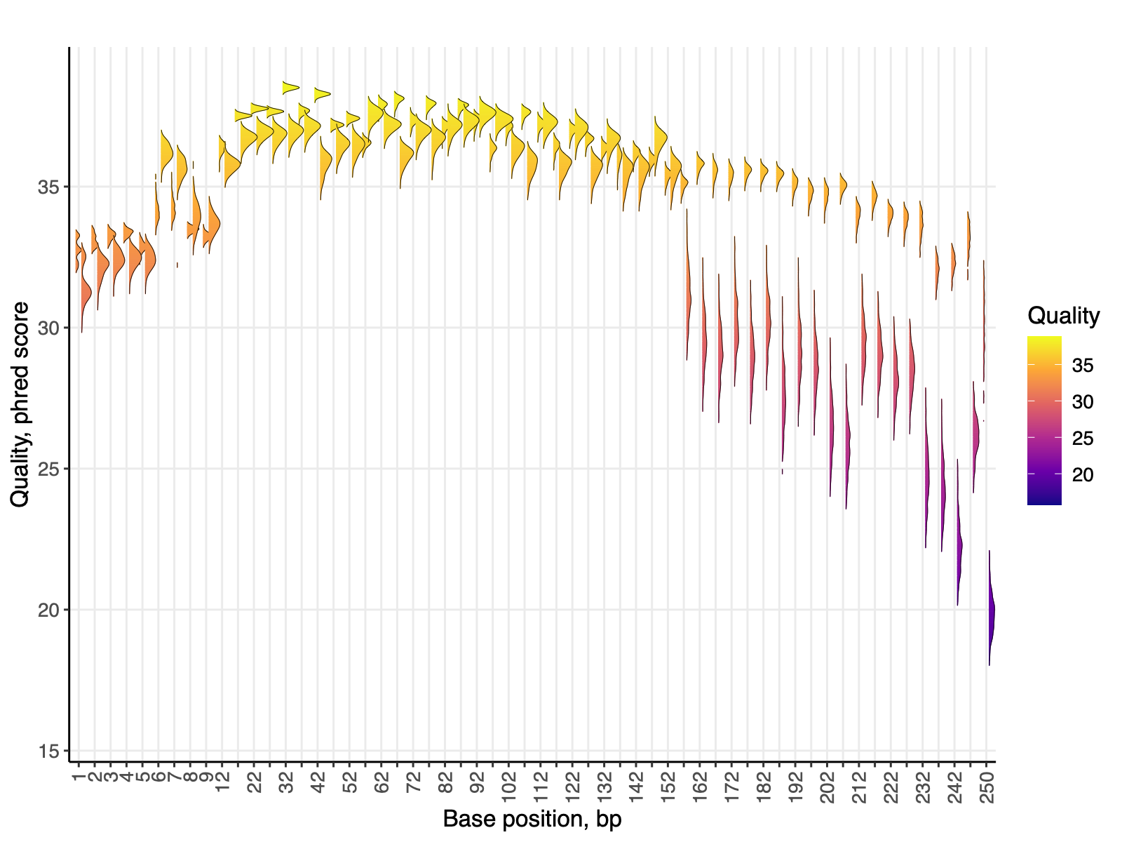
- The ridge plot below shows per-base quality scores across read positions. Each x-axis position includes two ridges: forward reads (left) and reverse reads (right)
- Interpretation: Forward reads have higher overall quality. Reverse read quality drops sharply around 157 bp, whereas forward reads remain consistently above a Phred score of 30
3.2 Adator trimming
- Optional primer/adapter trimming using cutadapt
$ cutadapt \
-g FORWARD_PRIMER_SEQ \
-G REVERSE_PRIMER_SEQ \
--discard-untrimmed \
-o sample_R1.trimmed.fastq.gz \
-p sample_R2.trimmed.fastq.gz \
sample_R1.fastq.gz sample_R2.fastq.gz3.3 Preparation in the R environment
- Set the working directory to import FASTQ files and save all outputs generated in this report
# Do not run
base_dir <- "WORKING_DIRECTORY" # path to your project folder
setwd(base_dir)3.4 Load R packages
- Required packages are listed in Section 2
library(dada2) # ASV inference and DADA2 pipeline functions
library(Biostrings) # DNA/RNA sequence handling (FASTA I/O, string ops)
library(ShortRead) # FASTQ input and quality assessment utilities
library(data.table) # fast, memory-efficient tabular data manipulation
library(ggplot2) # static plotting with the grammar of graphics
library(patchwork) # combine multiple ggplot figures into layouts
library(RColorBrewer) # color palettes (e.g., for plots/heatmaps)
library(plotly) # interactive versions of plots (hover/zoom)
library(phyloseq) # microbiome data structures + analysis/visualization3.5 Import FASTQ files
- Enumerate R1 files in the FASTQ directory, derive unique sample IDs from filenames, and (if paired-end) validate that each sample has a matching R2 file
- List FASTQ files, derive sample IDs, and validate paired-end matches
fastq_dir <- file.path(base_dir, "FASTQ", "raw")
r1_suffix <- "_R1.fastq.gz"
r2_suffix <- "_R2.fastq.gz"
r1_files <- sort(list.files(fastq_dir, pattern = paste0(r1_suffix, "$"), full.names = TRUE))
stop_if_not(length(r1_files) > 0, paste0("No R1 files matching '*", r1_suffix, "' found in: ", fastq_dir))
sample_ids <- vapply(r1_files, derive_sample_id_from_r1, character(1))
stop_if_not(!anyDuplicated(sample_ids), "Duplicate sample IDs derived from R1 filenames.")
names(r1_files) <- sample_ids
if (isTRUE(is_paired_end)) {
r2_files <- file.path(fastq_dir, paste0(sample_ids, r2_suffix))
missing_r2 <- !file.exists(r2_files)
stop_if_not(
!any(missing_r2),
paste0("Missing R2 files for: ", paste(sample_ids[missing_r2], collapse = ", "))
)
names(r2_files) <- sample_ids
} else {
r2_files <- character(0)
}3.6 Read quality
3.6.1 Raw reads
- Per-base quality profiles from the original demultiplexed FASTQs, before any trimming or filtering.
if (isTRUE(is_paired_end)) {
qp_raw <- filter_qp_inputs(unname(r1_files), unname(r2_files))
p_raw_R1 <- plotQualityProfile(qp_raw$R1, aggregate = TRUE) +
labs(subtitle = "Read 1")
p_raw_R2 <- plotQualityProfile(qp_raw$R2, aggregate = TRUE) +
labs(subtitle = "Read 2")
print(p_raw_R1 + p_raw_R2)
} else {
p_raw_R1 <- plotQualityProfile(unname(r1_files), aggregate = TRUE)
print(p_raw_R1)
}
3.6.2 After cutadapt
- Quality profiles after cutadapt processing, showing read quality after primer/adaptor removal and any configured trimming.
if (isTRUE(do_cutadapt)) {
cutadapt_dir <- base::file.path(base_dir, "FASTQ", "cutadapt")
ca_r1 <- sort(list.files(cutadapt_dir, pattern = paste0(r1_suffix, "$"), full.names = TRUE))
ca_ids <- vapply(ca_r1, derive_sample_id_from_r1, character(1))
if (isTRUE(is_paired_end)) {
ca_r2 <- file.path(cutadapt_dir, paste0(ca_ids, r2_suffix))
stop_if_not(all(file.exists(ca_r2)), "Missing some cutadapt R2 files.")
qp_afterqc <- filter_qp_inputs(ca_r1, ca_r2)
p_afterqc_R1 <- plotQualityProfile(qp_afterqc$R1, aggregate = TRUE) +
labs(subtitle = "After trimming (cutadapt) — Read 1")
p_afterqc_R2 <- plotQualityProfile(qp_afterqc$R2, aggregate = TRUE) +
labs(subtitle = "After trimming (cutadapt) — Read 2")
print(p_afterqc_R1 + p_afterqc_R2)
filt_in_r1 <- ca_r1
filt_in_r2 <- ca_r2
} else {
qp_afterqc <- list(R1 = ca_r1, R2 = NULL)
p_afterqc_R1 <- plotQualityProfile(qp_afterqc$R1, aggregate = TRUE) +
labs(subtitle = "After trimming (cutadapt) — Read 1")
print(p_afterqc_R1)
filt_in_r1 <- ca_r1
filt_in_r2 <- NULL
}
} else {
filt_in_r1 <- unname(r1_files)
filt_in_r2 <- if (isTRUE(is_paired_end)) unname(r2_files) else NULL
}
- Compared with the raw reads, this checkpoint highlights how cutadapt
affects:
- The effective read length distribution (reads may become shorter after trimming)
- The presence or reduction of low-quality tails (often improved if 3′ trimming is applied)
3.6.3 After filterAndTrim
- Quality profiles after DADA2
filterAndTrim(), reflecting the reads retained for denoising after quality-based trimming and filtering.
filter_trim_dir <- file.path(out_dir, "filter_and_trim")
dir_create(filter_trim_dir)
filt_out_r1 <- file.path(filter_trim_dir, paste0(sample_ids, r1_suffix))
if (isTRUE(is_paired_end)) {
filt_out_r2 <- file.path(filter_trim_dir, paste0(sample_ids, r2_suffix))
} else {
filt_out_r2 <- NULL
}
if (isTRUE(is_paired_end)) {
truncLen_vec <- c(as.integer(filt_truncLen_R1), as.integer(filt_truncLen_R2))
trimLeft_vec <- c(as.integer(filt_trimLeft_R1), as.integer(filt_trimLeft_R2))
maxEE_vec <- c(filt_maxEE_R1, filt_maxEE_R2)
filt_stats <- filterAndTrim(
fwd = filt_in_r1,
filt = filt_out_r1,
rev = filt_in_r2,
filt.rev = filt_out_r2,
truncLen = truncLen_vec,
trimLeft = trimLeft_vec,
maxN = filt_maxN,
maxEE = maxEE_vec,
truncQ = as.integer(filt_truncQ),
rm.phix = isTRUE(filt_rm_phix),
compress = isTRUE(filt_compress),
multithread = isTRUE(multithread),
matchIDs = isTRUE(filt_matchIDs)
)
} else {
filt_stats <- filterAndTrim(
fwd = filt_in_r1,
filt = filt_out_r1,
truncLen = as.integer(filt_truncLen_R1),
trimLeft = as.integer(filt_trimLeft_R1),
maxN = filt_maxN,
maxEE = filt_maxEE_R1,
truncQ = as.integer(filt_truncQ),
rm.phix = isTRUE(filt_rm_phix),
compress = isTRUE(filt_compress),
multithread = isTRUE(multithread)
)
}
filt_dt <- as.data.table(filt_stats, keep.rownames = "sample_id")
if (isTRUE(is_paired_end)) {
qp_after_filter <- filter_qp_inputs(filt_out_r1, filt_out_r2)
p_filt_R1 <- plotQualityProfile(qp_after_filter$R1, aggregate = TRUE) +
labs(subtitle = "After filterAndTrim — Read 1")
p_filt_R2 <- plotQualityProfile(qp_after_filter$R2, aggregate = TRUE) +
labs(subtitle = "After filterAndTrim — Read 2")
print(p_filt_R1 + p_filt_R2)
} else {
qp_after_filter <- list(R1 = filt_out_r1, R2 = NULL)
p_filt_R1 <- plotQualityProfile(filt_out_r1, aggregate = TRUE) +
labs(subtitle = "After filterAndTrim — Read 1")
print(p_filt_R1)
}
- These are the reads that will be used as input to denoising, so this checkpoint reflects what the algorithm actually sees.
3.7 Learn the error rates
- Builds an empirical sequencing error model from the quality-filtered reads
- DADA2 uses this model to distinguish true biological variants (ASVs) from sequencing errors during denoising
- Visualization: The learned substitution error rates from
learnErrors()- Each panel corresponds to a specific substitution type (e.g., A→C), showing how often one base is misread as another
- Axes and elements:
- X-axis: Phred quality score (Q). Higher Q means higher expected base-call accuracy
- Y-axis: Estimated probability of that substitution error on a log scale
- Points: Empirical error estimates derived from the observed data used to learn errors
- Lines: The fitted error model that DADA2 will use during denoising
- How to interpret a “good” plot:
- Monotonic trend: Error rates should generally decrease as Q increases (higher quality, fewer errors)
- Close agreement: Points and lines should be reasonably aligned, indicating the model fits the empirical signal
- Reasonable magnitude: At high Q scores, error rates should be very low; at lower Q scores, they should be higher
if (isTRUE(is_paired_end)) {
err_inputs <- exclude_negatives(qp_after_filter$R1, qp_after_filter$R2, neg_ids = neg_samples)
errF <- learnErrors(err_inputs$R1, nbases = learn_nbases, multithread = isTRUE(multithread))
errR <- learnErrors(err_inputs$R2, nbases = learn_nbases, multithread = isTRUE(multithread))
p_errF <- plotErrors(errF, nominalQ = TRUE) + labs(subtitle = "Forward (Read 1)")
p_errR <- plotErrors(errR, nominalQ = TRUE) + labs(subtitle = "Reverse (Read 2)")
print(p_errF + p_errR)
} else {
err_inputs <- exclude_negatives(qp_after_filter$R1, qp_after_filter$R1, neg_ids = neg_samples)
err_inputs$R2 <- NULL
errF <- learnErrors(err_inputs$R1, nbases = learn_nbases, multithread = isTRUE(multithread))
errR <- NULL
p_errF <- plotErrors(errF, nominalQ = TRUE) + labs(subtitle = "Forward (Read 1)")
print(p_errF)
}## Error learning inputs: R1 files = 330; R2 files = 330## 102086104 total bases in 406899 reads from 37 samples will be used for learning the error rates.
## 101865066 total bases in 406899 reads from 37 samples will be used for learning the error rates.
3.8 Dereplication and denoising
- Dereplication: compresses each sample into a set of
unique sequences and counts, which reduces redundancy and preserves
abundance information needed for inference.
- Efficiency: operating on unique sequences (rather than all reads) substantially reduces runtime and memory requirements.
- Accuracy: abundance-aware, error-model–based inference improves resolution beyond OTU clustering by separating closely related true variants from error-derived sequences.
- Denoising (the primary DADA2 step): uses the learned error models to distinguish true biological variants from sequencing errors and outputs per-sample ASV counts.
pool_arg <- map_pooling_mode(dada_pool)
derepF <- derepFastq(qp_after_filter$R1, verbose = FALSE)
names(derepF) <- sub(paste0(r1_suffix, "$"), "", basename(qp_after_filter$R1))
if (isTRUE(is_paired_end)) {
derepR <- derepFastq(qp_after_filter$R2, verbose = FALSE)
names(derepR) <- sub(paste0(r2_suffix, "$"), "", basename(qp_after_filter$R2))
} else {
derepR <- NULL
}
dadaF <- dada(derepF, err = errF, pool = pool_arg, multithread = isTRUE(multithread))
if (isTRUE(is_paired_end)) {
dadaR <- dada(derepR, err = errR, pool = pool_arg, multithread = isTRUE(multithread))
} else {
dadaR <- NULL
}
dadaF[[1]]
if (isTRUE(is_paired_end)) dadaR[[1]]## dada-class: object describing DADA2 denoising results
## 119 sequence variants were inferred from 2848 input unique sequences.
## Key parameters: OMEGA_A = 1e-40, OMEGA_C = 1e-40, BAND_SIZE = 16## dada-class: object describing DADA2 denoising results
## 100 sequence variants were inferred from 5217 input unique sequences.
## Key parameters: OMEGA_A = 1e-40, OMEGA_C = 1e-40, BAND_SIZE = 163.9 Merge paired reads
- Combines denoised forward and reverse sequences within each sample
by aligning their overlap
- Produces a single reconstructed amplicon sequence per variant (when reads overlap sufficiently), reducing read-end errors by requiring consistency across the overlap
- Applies merge criteria such as minimum overlap and allowed mismatches (if specified)
if (isTRUE(is_paired_end)) {
merge_args <- list(dadaF = dadaF, derepF = derepF, dadaR = dadaR, derepR = derepR, verbose = TRUE)
if (!is.null(merge_minOverlap)) merge_args$minOverlap <- as.integer(merge_minOverlap)
if (!is.null(merge_maxMismatch)) merge_args$maxMismatch <- as.integer(merge_maxMismatch)
mergers <- do.call(mergePairs, merge_args)
seqtab <- makeSequenceTable(mergers)
} else {
mergers <- NULL
seqtab <- makeSequenceTable(dadaF)
}
asv_seqs <- colnames(seqtab)
asv_ids <- sprintf("ASV%03d", seq_along(asv_seqs))
asv_map_dt <- data.table::data.table(
asv_id = asv_ids,
asv_sequence = asv_seqs,
asv_length = nchar(asv_seqs),
total_count = as.integer(colSums(seqtab))
)
# Inspect the matrix after replacing sequences in the column names
to_show <- seqtab
colnames(to_show) <- asv_ids
head(to_show[, c(1:5)])## ASV001 ASV002 ASV003 ASV004 ASV005
## F3D0 605 357 478 168 502
## F3D1 416 364 79 146 44
## F3D11 3302 1896 797 540 0
## F3D125 1110 676 767 476 852
## F3D13 2308 1870 1049 1225 306
## F3D141 462 384 543 199 354# Inspect sequence table dimensions: (n_samples x n_ASVs)
dim(seqtab)## [1] 330 420# Inspect the first column name
colnames(seqtab)[1] # ASV001## [1] "TACGGAGGATGCGAGCGTTATCCGGATTTATTGGGTTTAAAGGGTGCGCAGGCGGAAGATCAAGTCAGCGGTAAAATTGAGAGGCTCAACCTCTTCGAGCCGTTGAAACTGGTTTTCTTGAGTGAGCGAGAAGTATGCGGAATGCGTGGTGTAGCGGTGAAATGCATAGATATCACGCAGAACTCCGATTGCGAAGGCAGCATACCGGCGCTCAACTGACGCTCATGCACGAAAGTGTGGGTATCGAACAGG"# Inspect distribution of sequence lengths
table(nchar(getSequences(seqtab)))##
## 251 252 253 254 255
## 1 77 329 9 43.10 Remove chimeras
- Removes likely PCR chimeras (artificial sequences formed by
recombination of two true templates during amplification) from the ASV
table using
removeBimeraDenovo() - This step reduces false-positive ASVs and improves downstream interpretation
seqtab_nochim <- removeBimeraDenovo(
seqtab,
method = chimera_method,
multithread = isTRUE(multithread),
verbose = TRUE
)## Identified 66 bimeras out of 420 input sequences.3.11 Read retention overview
3.11.1 Statistics tracking and export
- Record the number of reads removed at each step and export stats with sample metadata
- All exported files are available in the Downloads section below
filt_dt_clean <- copy(filt_dt)
filt_dt_clean[, sample_id := sub(paste0(r1_suffix, "$"), "", basename(sample_id))]
setkey(filt_dt_clean, sample_id)
track_dt <- data.table(
sample_id = names(dadaF),
denoised_F = vapply(dadaF, getN, integer(1)),
denoised_R = if (isTRUE(is_paired_end)) vapply(dadaR, getN, integer(1)) else NA_integer_,
merged = rowSums(seqtab, na.rm = TRUE),
nonchim = rowSums(seqtab_nochim, na.rm = TRUE)
)
track_dt <- merge(
track_dt,
filt_dt_clean[, .(sample_id, reads_in = reads.in, reads_filtered = reads.out)],
by = "sample_id",
all.x = TRUE
)
setcolorder(
track_dt,
c("sample_id", "reads_in", "reads_filtered", "denoised_F", "denoised_R", "merged", "nonchim")
)
track_dt <- as.data.table(track_dt)
track_dt[, denoised := if (isTRUE(is_paired_end)) pmin(denoised_F, denoised_R) else denoised_F]
track_dt[, sex := fifelse(
grepl("^F", sample_id), "Female",
fifelse(grepl("^M", sample_id), "Male", NA_character_)
)]
track_dt[, day := as.integer(sub(".*D", "", sample_id))]
track_dt[, stage := fifelse(
day <= 50L, "Early",
fifelse(day >= 100L, "Late", NA_character_)
)]
track_dt[, group := factor(
paste(stage, sex, sep = " + "),
levels = c("Early + Male", "Early + Female", "Late + Male", "Late + Female")
)]
track_dt[, pct_remaining_final := 100 * (nonchim / reads_in)]
head(track_dt)## Key: <sample_id>
## sample_id reads_in reads_filtered denoised_F denoised_R merged nonchim
## <char> <num> <num> <int> <int> <num> <num>
## 1: F3D0 7793 7733 7486 7094 6060 6060
## 2: F3D1 5869 5829 5657 5453 5083 5083
## 3: F3D11 17790 17670 17322 16105 14284 14089
## 4: F3D125 12674 12609 12294 11471 9383 9340
## 5: F3D13 17277 17172 16905 15613 13953 13676
## 6: F3D141 5958 5926 5733 5302 4490 4490
## denoised sex day stage group pct_remaining_final
## <int> <char> <int> <char> <fctr> <num>
## 1: 7094 Female 0 Early Early + Female 77.76209
## 2: 5453 Female 1 Early Early + Female 86.60760
## 3: 16105 Female 11 Early Early + Female 79.19618
## 4: 11471 Female 125 Late Late + Female 73.69418
## 5: 15613 Female 13 Early Early + Female 79.15726
## 6: 5302 Female 141 Late Late + Female 75.360863.11.2 Mean read retention summary
- Mean read retention from raw input to the final non-chimeric ASV table, reported as percent retained versus excluded across all samples
mean_remaining <- mean(track_dt$pct_remaining_final, na.rm = TRUE)
mean_excluded <- 100 - mean_remaining
bar1_dt <- data.table(
label = "Raw to final",
status = factor(c("Remaining", "Excluded"), levels = c("Remaining", "Excluded")),
pct = c(mean_remaining, mean_excluded)
)
ggplot(bar1_dt, aes(x = label, y = pct, fill = status)) +
geom_col(width = 0.6) +
coord_flip() +
geom_text(
aes(label = sprintf("%.1f%%", pct)),
position = position_stack(vjust = 0.5),
size = 4
) +
scale_fill_manual(values = c("Remaining" = "steelblue", "Excluded" = "grey60")) +
scale_y_continuous(limits = c(0, 100), expand = expansion(mult = c(0, 0.02))) +
labs(
title = NULL,
x = NULL,
y = "Percentage of reads",
fill = NULL
) +
theme_classic(base_size = 12) +
theme(
legend.position = "bottom",
text = element_text(size = 12)
)
3.11.3 Read retention by time and group
- Mean remaining reads at each major checkpoint, summarized across the four groups (Early/Late × Female/Male) to highlight where reads are primarily lost and whether retention differs by group.
steps_to_plot <- c("reads_in", "reads_filtered", "denoised", "merged", "nonchim")
step_labels <- c(
reads_in = "Raw reads",
reads_filtered = "After filterAndTrim",
denoised = "After denoising",
merged = "After merging pairs",
nonchim = "After chimera removal"
)
plot_long <- melt(
track_dt[, c("sample_id", "group", steps_to_plot), with = FALSE],
id.vars = c("sample_id", "group"),
variable.name = "step",
value.name = "remaining_reads"
)
plot_long[, step := factor(step, levels = steps_to_plot, labels = unname(step_labels[steps_to_plot]))]
sum_dt <- plot_long[, .(remaining_reads = mean(remaining_reads, na.rm = TRUE)), by = .(step, group)]
y_max <- max(sum_dt$remaining_reads, na.rm = TRUE)
step_cols <- brewer.pal(n = 5, name = "Dark2")
names(step_cols) <- levels(sum_dt$step)
ggplot(sum_dt, aes(x = step, y = remaining_reads, fill = step)) +
geom_col(width = 0.75) +
facet_wrap(~group, ncol = 2, scales = "fixed") +
scale_y_continuous(
limits = c(0, y_max),
expand = expansion(mult = c(0, 0.05))
) +
scale_fill_manual(values = step_cols) +
labs(
title = NULL,
x = NULL,
y = "Remaining reads (mean within group)",
fill = NULL
) +
theme_classic(base_size = 12) +
theme(
legend.position = "bottom",
text = element_text(size = 12),
axis.text.x = element_blank(),
axis.ticks.x = element_blank()
)
3.12 ASV composition snapshot
3.12.1 ASV prevalence and abundance
- Core: All remaining ASVs outside the
low-abundance/low-prevalence region. These are comparatively
well-supported variants detected in more samples and/or at higher total
counts, and therefore most strongly influence downstream community
summaries.
- Intermediate: ASVs in the lowest
10% of both abundance and prevalence, excluding the
“Rare” set. These are low-to-moderate support variants that occur in a
limited subset of samples and may reflect condition-specific taxa,
low-level carryover, or biologically uncommon members.
- Rare: ASVs in the lowest 5% of both total abundance (summed counts across all samples) and prevalence (number of samples detected). These represent low-support, sparsely observed variants that contribute minimally to the overall read pool.
n_samples <- nrow(seqtab_nochim)
n_asvs <- ncol(seqtab_nochim)
prev_abund_dt <- data.table(
asv_sequence = colnames(seqtab_nochim),
abundance_total_count = as.integer(colSums(seqtab_nochim)),
prevalence_n_samples = as.integer(colSums(seqtab_nochim >= presence_threshold))
)
asv_map_sub <- unique(asv_map_dt[, .(asv_id, asv_sequence, asv_length)])
setkey(asv_map_sub, asv_sequence)
setkey(prev_abund_dt, asv_sequence)
prev_abund_dt <- asv_map_sub[prev_abund_dt]
prevalence_cutoff_rare <- as.numeric(quantile(
prev_abund_dt$prevalence_n_samples,
probs = p_rare, na.rm = TRUE, type = 7
))
prevalence_cutoff_intermediate <- as.numeric(quantile(
prev_abund_dt$prevalence_n_samples,
probs = p_intermediate, na.rm = TRUE, type = 7
))
abundance_cutoff_rare <- as.numeric(quantile(
prev_abund_dt$abundance_total_count,
probs = p_rare, na.rm = TRUE, type = 7
))
abundance_cutoff_intermediate <- as.numeric(quantile(
prev_abund_dt$abundance_total_count,
probs = p_intermediate, na.rm = TRUE, type = 7
))
prevalence_cutoff_rare_i <- floor(prevalence_cutoff_rare)
prevalence_cutoff_intermediate_i <- floor(prevalence_cutoff_intermediate)
abundance_cutoff_rare_i <- floor(abundance_cutoff_rare)
abundance_cutoff_intermediate_i <- floor(abundance_cutoff_intermediate)
prev_abund_dt[, class := "Core"]
prev_abund_dt[
prevalence_n_samples <= prevalence_cutoff_intermediate_i &
abundance_total_count <= abundance_cutoff_intermediate_i,
class := "Intermediate"
]
prev_abund_dt[
prevalence_n_samples <= prevalence_cutoff_rare_i &
abundance_total_count <= abundance_cutoff_rare_i,
class := "Rare"
]
prev_abund_dt[, class := factor(class, levels = c("Rare", "Intermediate", "Core"))]
n_rare <- sum(prev_abund_dt$class == "Rare")
n_int <- sum(prev_abund_dt$class == "Intermediate")
n_core <- sum(prev_abund_dt$class == "Core")
summary_sentence <- sprintf(
"Total ASVs: %d in %d samples. Rare: %d; Intermediate: %d; Core: %d",
n_asvs, n_samples, n_rare, n_int, n_core
)
sample_ids <- rownames(seqtab_nochim)
top_sample_str <- vapply(seq_len(ncol(seqtab_nochim)), function(j) {
col <- seqtab_nochim[, j]
idx <- which(col > 0)
if (length(idx) == 0) {
return("None (ASV not observed)")
}
ord <- idx[order(col[idx], decreasing = TRUE)]
ord <- ord[seq_len(min(length(ord), top_samples_in_hover))]
paste0(sample_ids[ord], " (", as.integer(col[ord]), ")", collapse = "; ")
}, character(1))
prev_abund_dt[, top_samples := top_sample_str]
prev_abund_dt[, hover := paste0(
"ASV: ", asv_id,
"<br>Class: ", as.character(class),
"<br>Abundance (total count): ", abundance_total_count,
"<br>Prevalence (n samples): ", prevalence_n_samples,
"<br>ASV length (bp): ", ifelse(is.na(asv_length), "NA", as.character(asv_length)),
"<br>Top sample(s): ", top_samples
)]
color_map <- c("Rare" = "grey60", "Intermediate" = "goldenrod2", "Core" = "dodgerblue3")
p_prev_abund <- plot_ly(
data = prev_abund_dt,
x = ~abundance_total_count,
y = ~prevalence_n_samples,
type = "scatter",
mode = "markers",
color = ~class,
colors = color_map,
text = ~hover,
hoverinfo = "text"
) |>
layout(
title = list(text = summary_sentence),
xaxis = list(title = "Abundance (total count; log10)", type = "log"),
yaxis = list(title = "Prevalence (number of samples)", rangemode = "tozero"),
legend = list(
orientation = "h",
x = 0.5, xanchor = "center",
y = -0.1, yanchor = "top"
),
hoverlabel = list(align = "left")
)
p_prev_abund3.12.2 ASV length distribution
- Two complementary views:
- (left) Histogram of ASV lengths (counts of ASVs per length)
- (right) Abundance-weighted histogram (sum of total_count per length)
len_counts_dt <- asv_map_dt[, .(n_asvs = .N), by = .(asv_length)]
setorder(len_counts_dt, asv_length)
p_len_count <- ggplot(len_counts_dt, aes(x = asv_length, y = n_asvs)) +
geom_col() +
labs(
title = NULL,
x = "ASV length (bp)",
y = "Number of ASVs"
) +
theme_classic(base_size = 12)
len_abund_dt <- asv_map_dt[, .(total_reads = sum(as.integer(total_count), na.rm = TRUE)), by = .(asv_length)]
setorder(len_abund_dt, asv_length)
p_len_abund <- ggplot(len_abund_dt, aes(x = asv_length, y = total_reads)) +
geom_col() +
scale_y_log10() +
labs(
title = NULL,
x = "ASV length (bp)",
y = "Total reads assigned to ASVs (log10)"
) +
theme_classic(base_size = 12)
print(p_len_count + p_len_abund)
4 Taxonomy assignment
- DADA2 will serve as the primary method because it denoises amplicon reads into high-confidence ASVs and removes artifacts (e.g., sequencing errors and chimeras)
- VSEARCH will be used as a complementary step to provide post hoc, reference-based confirmation and annotation of representative ASV sequences against curated databases
4.1 DADA2’s taxonomy assignment
- The DADA2 function
assignTaxonomy()provides a built-in implementation of the naïve Bayesian classifier for taxonomic assignment - Multiple reference DBs were used to assign taxonomy to ASVs; the below shows an example using SILVA, while taxonomy assignments from the other databases are provided in the Download section
- DADA2-formatted training fasta file was downloaded from
Taxonomic
reference data
- SILVA: Broad coverage across Bacteria, Archaea, and Eukaryota (SSU rRNA (16S/18S) and LSU rRNA)
- RDP: rRNA sequences plus the RDP Classifier ecosystem (16S (Bacteria/Archaea) and fungal 28S)
- GreenGenes2: Unifies 16S and genomic data in one reference tree (16S integrated with genome phylogeny)
# Set the file paths to your taxonomy reference files
tax_train_fasta <- "path/to/trainset.fa"
tax_species_fasta <- "path/to/assignSpecies.fa"tax_mat <- dada2::assignTaxonomy(
seqtab_nochim,
refFasta = tax_train_fasta,
multithrea = isTRUE(multithread),
tryRC = TRUE
)
tax_mat <- dada2::addSpecies(tax_mat, refFasta = tax_species_fasta, allowMultiple = TRUE)
to_show <- tax_mat # Removing sequence rownames for display only
rownames(to_show) <- NULL
head(to_show)## Kingdom Phylum Class Order Family
## [1,] "Bacteria" "Bacteroidota" "Bacteroidia" "Bacteroidales" "Muribaculaceae"
## [2,] "Bacteria" "Bacteroidota" "Bacteroidia" "Bacteroidales" "Muribaculaceae"
## [3,] "Bacteria" "Bacteroidota" "Bacteroidia" "Bacteroidales" "Muribaculaceae"
## [4,] "Bacteria" "Bacteroidota" "Bacteroidia" "Bacteroidales" "Bacteroidaceae"
## [5,] "Bacteria" "Bacteroidota" "Bacteroidia" "Bacteroidales" "Muribaculaceae"
## [6,] "Bacteria" "Bacteroidota" "Bacteroidia" "Bacteroidales" "Rikenellaceae"
## Genus Species
## [1,] NA NA
## [2,] NA NA
## [3,] NA NA
## [4,] "Bacteroides" "acidifaciens/caecimuris"
## [5,] NA NA
## [6,] "Alistipes" NA4.2 GTDB-based annotation with VSEARCH
- Runs a GTDB reference search by matching DADA2 ASV sequences to the GTDB database with VSEARCH
- Adds GTDB hits to the ASV annotation table and exports unmatched ASVs to a separate FASTA file
4.2.1 Run VSEARCH
- VSEARCH (macOS; v2.30.1) was installed via Homebrew and executed from the terminal:
$ vsearch --usearch_global asv_sequences.fasta \
--db GTDB_bac120_arc53_ssu_r220_fullTaxo.fa \
--notrunclabels \
--userout Vsearch_GTDB_selected.tsv \
--userfields query+target+id \
--uc Vsearch_GTDB_raw.uc \
--id 0.9 \
--iddef 0 \
--maxaccepts 30 \
--top_hits_only \
--strand both \
--threads 1 \
--log log.txt4.2.2 Summarize GTDB hits
- GTDB hits were merged with ASV metadata to generate an annotated results table, available in the Download section below
$ head Vsearch_GTDB_hits.tsv
asv_id asv_seq asv_length total_count gtdb_hit identity
ASV001 TACGGAGGATGCGAGCGTTATCCGGA... 252 278298 Bacteria;Bacteroidota;Bacteroidia;Bacteroidales;Muribaculaceae;Duncaniella;Duncaniella_muris(RS_GCF_003024805_1 100
ASV002 TACGGAGGATGCGAGCGTTATCCGGA... 252 237358 Bacteria;Bacteroidota;Bacteroidia;Bacteroidales;Muribaculaceae;Duncaniella;Duncaniella_freteri(RS_GCF_004766125_1 95.2
ASV003 TACGGAGGATGCGAGCGTTATCCGGA... 252 198254 Bacteria;Bacteroidota;Bacteroidia;Bacteroidales;Muribaculaceae;UBA7173;UBA7173_sp013316675(GB_GCA_910575545_1 93.7
ASV004 TACGGAGGATCCGAGCGTTATCCGGA... 253 168783 Bacteria;Bacteroidota;Bacteroidia;Bacteroidales;Bacteroidaceae;Bacteroides;Bacteroides_caecimuris(RS_GCF_001688725_2 100
ASV005 TACGGAGGATGCGAGCGTTATCCGGA... 252 141946 Bacteria;Bacteroidota;Bacteroidia;Bacteroidales;Muribaculaceae;UBA7173;UBA7173_sp001689685(GB_GCA_910575615_1 99.6
ASV006 TACGGAGGATTCAAGCGTTATCCGGA... 253 110922 Bacteria;Bacteroidota;Bacteroidia;Bacteroidales;Rikenellaceae;Alistipes;Alistipes_sp003979135(GB_GCA_948603215_1 100
ASV007 TACGGAGGATGCGAGCGTTATCCGGA... 252 102123 Bacteria;Bacteroidota;Bacteroidia;Bacteroidales;Muribaculaceae;JAGBWK01;JAGBWK01_sp004102805(GB_GCA_004102805_1 96.8
ASV008 TACGGAGGATGCGAGCGTTATCCGGA... 252 98814 Bacteria;Bacteroidota;Bacteroidia;Bacteroidales;Muribaculaceae;Paramuribaculum;Paramuribaculum_sp001689565(GB_GCA_003762715_1 97.2
ASV009 TACGGAGGATGCGAGCGTTATCCGGA... 252 95637 Bacteria;Bacteroidota;Bacteroidia;Bacteroidales;Muribaculaceae;JAGBWK01;JAGBWK01_sp004102805(GB_GCA_004102805_1 95.65 Analysis
- The phyloseq R package provides a robust framework for downstream microbiome analysis and visualization, and the scripts used here were adapted from the phyloseq tutorial
- Results and visualizations are reported based on SILVA for consistency; however, taxonomy assignments from the other databases may be loaded to reproduce the same workflow using the scripts provided below
5.1 Format conversion
- First, the DADA2 output object (i.e.,
seqtab_nochim) needs to be converted into a phyloseq object.
sample_ids <- rownames(seqtab_nochim)
subject_raw <- sapply(strsplit(sample_ids, "D"), `[`, 1)
sex <- substr(subject_raw, 1, 1)
day <- as.integer(sapply(strsplit(sample_ids, "D"), `[`, 2))
sam_df <- data.frame(
Subject = sample_ids,
Sex = factor(sex, levels = c("M", "F")),
Day = day
)
sam_df$Group <- factor(ifelse(sam_df$Day > 100, "Late", "Early"),
levels = c("Early", "Late"),
labels = c("E", "L")
)
sam_df$Category <- factor(paste0(sam_df$Group, "_", sam_df$Sex),
levels = c("E_M", "E_F", "L_M", "L_F")
)
rownames(sam_df) <- sample_ids
ps <- phyloseq(
otu_table(seqtab_nochim, taxa_are_rows = FALSE),
sample_data(sam_df),
tax_table(tax_mat)
)
dna <- DNAStringSet(taxa_names(ps))
names(dna) <- taxa_names(ps)
ps <- merge_phyloseq(ps, dna)
taxa_names(ps) <- sprintf("ASV%03d", seq(ntaxa(ps)))
ps## phyloseq-class experiment-level object
## otu_table() OTU Table: [ 354 taxa and 330 samples ]
## sample_data() Sample Data: [ 330 samples by 5 sample variables ]
## tax_table() Taxonomy Table: [ 354 taxa by 7 taxonomic ranks ]
## refseq() DNAStringSet: [ 354 reference sequences ]5.2 Alpha diversity over time
- Visualize within-sample diversity using Shannon and Simpson indices across sampling Day, with points colored by Group (Early/Late) and shaped by Sex (Male/Female)
5.2.1 Group highlighted by color
plot_richness(ps,
x = "Day", measures = c("Shannon", "Simpson"),
color = "Group", shape = "Sex"
) +
theme_bw() +
scale_color_manual(values = group_cols) +
geom_point(size = 3)
5.2.2 Sex highlighted by color
plot_richness(ps,
x = "Day", measures = c("Shannon", "Simpson"),
shape = "Group", color = "Sex"
) +
theme_bw() +
scale_color_manual(values = sex_cols) +
geom_point(size = 3)
5.3 Beta diversity
5.3.1 Non-metric Multidimensional Scaling
- Assess between-sample community differences using Bray–Curtis distances on relative-abundance data and visualize them with NMDS, with points colored by Group (Early/Late) and shaped by Sex (Male/Female)
ps_nz <- prune_samples(sample_sums(ps) > 0, ps)
otu <- as(otu_table(ps_nz), "matrix")
if (taxa_are_rows(ps_nz)) otu <- t(otu)
otu[!is.finite(otu)] <- 0
otu_table(ps_nz) <- otu_table(otu, taxa_are_rows = FALSE)
ps_prop <- transform_sample_counts(ps_nz, function(x) x / sum(x))
nmds_bray <- ordinate(ps_prop, method = "NMDS", distance = "bray", trace = 0)
p_ordi <- plot_ordination(ps_prop, nmds_bray, color = "Group", shape = "Sex") +
geom_point(
aes(
text = paste0(
"Subject: ", Subject,
"<br>Group: ", Group,
"<br>Sex: ", Sex
)
),
size = 3
) +
theme_bw() +
scale_color_manual(values = group_cols)
ggplotly(p_ordi, tooltip = "text")5.3.2 Bray–Curtis distance heatmap
- Compute Bray–Curtis sample-to-sample distances and visualize them as a PCoA-ordered heatmap, with samples labeled and ordered by Day and annotated by Category (Group × Sex)
p_hm <- plot_heatmap(
ps_nz,
distance = "bray",
method = "PCoA",
sample.label = "Subject",
sample.order = "Subject",
sample.color = "Category"
) +
scale_fill_viridis_c(option = "C") +
guides(
fill = guide_colorbar(
barwidth = unit(10, "cm"),
barheight = unit(0.35, "cm"),
title.position = "top"
),
colour = guide_legend(nrow = 2, byrow = TRUE)
) +
theme(
legend.position = "bottom",
legend.box = "vertical",
legend.text = element_text(size = 9),
legend.title = element_text(size = 9),
legend.spacing.x = unit(0.3, "cm"),
axis.text.x = element_text(angle = 90, vjust = 0.5, hjust = 1),
axis.text.y = element_text(size = 9)
)
p_hm
5.4 Taxonomic relative abundance
- Plot the top 20 most abundant ASVs as relative abundance bar charts, aggregated and colored by Taxa, and faceted by Group (Early/Late) and Sex (Male/Female) across sampling days
top <- names(sort(taxa_sums(ps), decreasing = TRUE))[1:20]
ps_top <- transform_sample_counts(ps, function(OTU) OTU / sum(OTU))
ps_top <- prune_taxa(top, ps_top)
df_plot <- psmelt(ps_top)
df_plot$Family <- as.character(df_plot$Family)
df_plot$Family[is.na(df_plot$Family) | df_plot$Family == ""] <- "Unassigned"
dt <- as.data.table(df_plot)
dt_sum <- dt[, .(Abundance = mean(Abundance, na.rm = TRUE)), by = .(Category, Family)]
dt_sum[, Abundance := Abundance / sum(Abundance), by = Category]
ggplot(dt_sum, aes(x = Category, y = Abundance, fill = Family)) +
geom_col(color = NA) +
scale_y_continuous(limits = c(0, 1), labels = scales::percent) +
scale_fill_brewer(palette = "Set2", drop = FALSE) +
theme_bw() +
theme(
legend.position = "bottom",
axis.text.x = element_text(angle = 90, vjust = 0, hjust = 1)
) +
coord_flip()
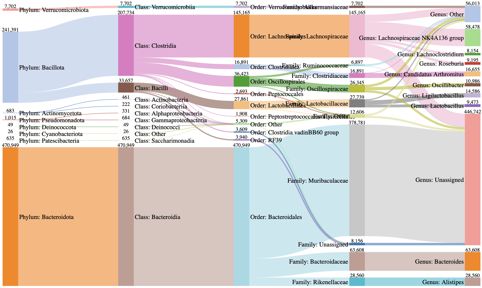
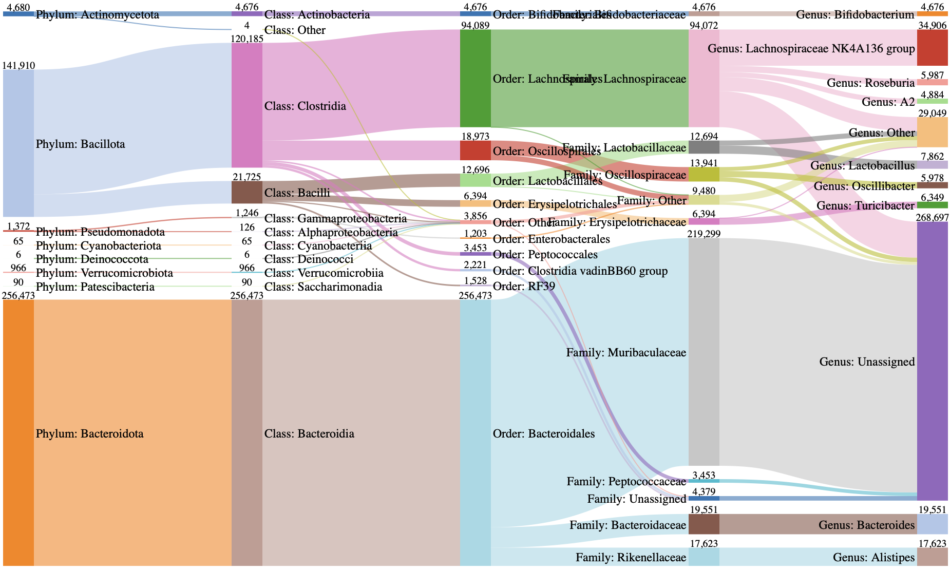
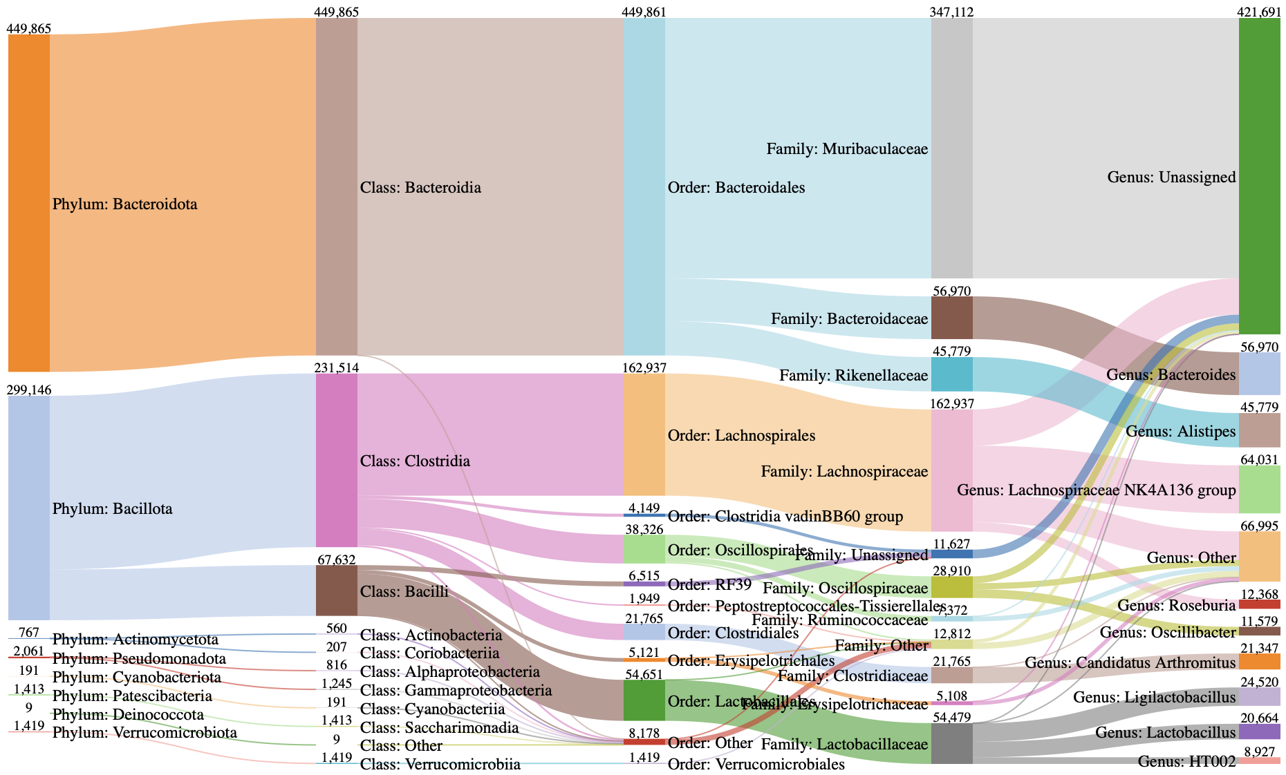
5.5 Taxonomic lineage profiles by category
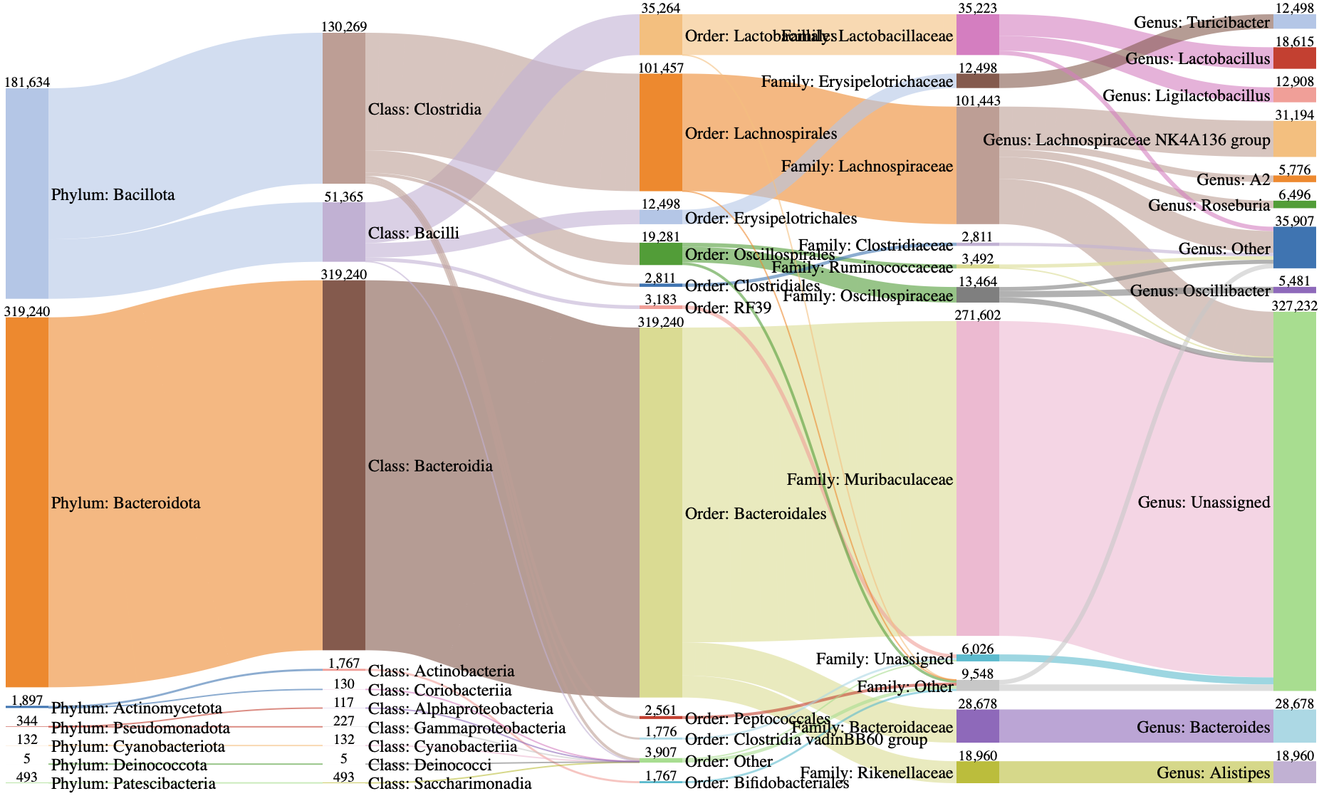
- Taxonomic composition is summarized as lineage-level flows from higher to lower ranks for each category, enabling rapid comparison of dominant clades and where group-specific differences emerge along the taxonomic hierarchy
- Click an image to view an enlarged version
|
| ||
| Sex | Early | Late |
|---|---|---|
|
| ||
| Male |
|
|
| Female |
|
|
|
| ||
6 Download
6.1 Preprocessing
- read_tracking.tsv: Per-sample read count tracking table showing how many reads remain at each pipeline step
- seqtab_asv_ids.tsv: ASV count table with samples as rows and ASV IDs as columns
- asv_id_map.tsv: Tab-delimited mapping of ASV IDs to their corresponding DNA sequences
- asv_sequences.fasta: FASTA file containing all unique ASV sequences (one record per ASV)
- seqtab_raw.rds: R object for reproducibility and reloading without re-running earlier steps
6.2 Taxonomy classification
- DADA2_taxonomy_matrix_SILVA.rds: R object containing the DADA2 taxonomic assignment matrix
- DADA2_taxonomy_matrix_RDP.rds: R object containing the DADA2 taxonomic assignment matrix
- DADA2_taxonomy_matrix_GG2.rds: R object containing the DADA2 taxonomic assignment matrix
- DADA2_phyloseq_obj.rds: R phyloseq object integrating the ASV table, sample metadata, taxonomy, and sequences
- Vsearch_GTDB_hits.tsv: Tab-delimited table of vsearch top-hit results against the GTDB reference
7 Research reproducibility
7.1 Parameters used in this analysis
| Parameter | Description | This analysis | Default |
|---|---|---|---|
| filt_truncLen_R1 | Truncate reads to a fixed length | 0 | 0 |
| filt_trimLeft_R1 | Remove a fixed number of bases from the 5′ end | 0 | 0 |
| filt_truncQ | Truncate reads at the first position with quality score ≤ this threshold | 2 | 2 |
| filt_maxEE_R1 | Discard reads with expected errors exceeding this threshold | Inf | Inf |
| filt_maxN | Discard reads with more than this number of ambiguous bases (N) | 0 | 0 |
| filt_rm_phix | Remove reads matching PhiX if present | TRUE | TRUE |
| learn_nbases | Number of bases used to learn the error model | 1e+08 | 1e+08 |
| dada_pool | Pooling strategy for sample inference | none | none |
| chimera_method | Chimera removal approach used during ASV inference | consensus | consensus |
7.2 Session info
## ─ Session info ───────────────────────────────────────────────────────────────────────────────────────
## setting value
## version R version 4.5.1 (2025-06-13)
## os macOS Tahoe 26.2
## system aarch64, darwin20
## ui X11
## language (EN)
## collate en_CA.UTF-8
## ctype en_CA.UTF-8
## tz America/Edmonton
## date 2026-01-18
##
## ─ Packages ───────────────────────────────────────────────────────────────────────────────────────────
## package * version date (UTC) lib source
## Biobase * 2.68.0 2025-04-15 [1] Bioconductor 3.21 (R 4.5.0)
## BiocGenerics * 0.54.1 2025-10-09 [1] Bioconductor 3.21 (R 4.5.1)
## BiocParallel * 1.42.2 2025-09-11 [1] Bioconductor 3.21 (R 4.5.1)
## Biostrings * 2.76.0 2025-04-15 [1] Bioconductor 3.21 (R 4.5.0)
## dada2 * 1.36.0 2025-04-15 [1] Bioconductor 3.21 (R 4.5.0)
## data.table * 1.18.0 2025-12-24 [1] CRAN (R 4.5.2)
## generics * 0.1.4 2025-05-09 [1] CRAN (R 4.5.0)
## GenomeInfoDb * 1.44.3 2025-09-18 [1] Bioconductor 3.21 (R 4.5.1)
## GenomicAlignments * 1.44.0 2025-04-15 [1] Bioconductor 3.21 (R 4.5.0)
## GenomicRanges * 1.60.0 2025-04-15 [1] Bioconductor 3.21 (R 4.5.0)
## ggplot2 * 4.0.1 2025-11-14 [1] CRAN (R 4.5.2)
## IRanges * 2.42.0 2025-04-15 [1] Bioconductor 3.21 (R 4.5.0)
## MatrixGenerics * 1.20.0 2025-04-15 [1] Bioconductor 3.21 (R 4.5.0)
## matrixStats * 1.5.0 2025-01-07 [1] CRAN (R 4.5.0)
## patchwork * 1.3.2 2025-08-25 [1] CRAN (R 4.5.0)
## phyloseq * 1.52.0 2025-04-15 [1] Bioconductor 3.21 (R 4.5.1)
## plotly * 4.11.0 2025-06-19 [1] CRAN (R 4.5.0)
## RColorBrewer * 1.1-3 2022-04-03 [1] CRAN (R 4.5.0)
## Rcpp * 1.1.0 2025-07-02 [1] CRAN (R 4.5.0)
## Rsamtools * 2.24.1 2025-09-04 [1] Bioconductor 3.21 (R 4.5.1)
## S4Vectors * 0.46.0 2025-04-15 [1] Bioconductor 3.21 (R 4.5.0)
## ShortRead * 1.66.0 2025-04-15 [1] Bioconductor 3.21 (R 4.5.0)
## SummarizedExperiment * 1.38.1 2025-04-28 [1] Bioconductor 3.21 (R 4.5.0)
## XVector * 0.48.0 2025-04-15 [1] Bioconductor 3.21 (R 4.5.0)
##
## [1] /Library/Frameworks/R.framework/Versions/4.5-arm64/Resources/library
## * ── Packages attached to the search path.
##
## ──────────────────────────────────────────────────────────────────────────────────────────────────────