[Session 5] From Expression Signatures to Prediction:
Building and Evaluating a Sample Classifier

1 Introduction

1.1 Study overview and prediction task

Session 4 asked which genes differ, on average, between Parkinson’s disease (PD) and control samples. This session asks a distinct predictive question: given a brain sample that the model has never encountered, can its diagnosis be inferred from gene expression?
We reproduce Figure 1g, the final panel of Figure 1 and the only panel not addressed in Session 4.
The paper reports:

“Using a group of 70% of our control and donor PD caudates as a training dataset, we discovered a set of 19 classifier genes which identified clinical diagnosis with 86% accuracy. The same set of classifier genes identified clinical diagnosis in the putamen with 90% accuracy.”

The key published results are therefore 19 classifier genes, 86% accuracy in held-out caudate samples, and 90% accuracy in putamen samples.
The transfer to putamen is especially important. The classifier is trained only on caudate samples and then evaluated in a different brain region. Successful transfer suggests that the model captures a disease-associated expression pattern rather than a signal specific to one tissue subset.

1.2 Published workflow and analytical approach

The Methods describe the following procedure:

“To identify classifier genes for PD and control patients, we used the MLSeq Bioconductor package (version 2.12.0) to implement a nearest shrunken centroid classifier on the voom variance stabilized caudate RNA-seq data. We used 70% of all samples as our training set and 30% as our test dataset. The accuracy of models on test data were recorded. Following this, the accuracy of the caudate classifier was also assessed in the putamen.”

# Demonstration only; do not run
method     = "voomNSC"
normalize  = "deseq"
ref        = "CTRL"
control    = MLSeq::voomControl(method = "repeatedcv", number = 5, repeats = 10, tuneLength = 10)
set.seed(1710)

1.3 How the voomNSC classifier works

voomNSC combines two ideas:
- voom transforms count data to log₂ counts per million and models the mean–variance relationship so that linear modelling methods can be applied appropriately.
- Nearest shrunken centroids (NSC) estimates a class-specific expression centroid for each gene in PD and control samples, then assigns a new sample to the class whose centroid is closest.
Shrinkage pulls class-specific centroids toward the overall centroid. Genes with weak class separation are shrunk to zero difference and no longer contribute to prediction.
Feature selection is embedded within model fitting. Cross-validation selects the shrinkage threshold, and the genes that retain non-zero class differences form the final predictive signature. The published set of 19 genes is an output of this tuning procedure rather than a prespecified target.

1.4 Environment

This session runs in R and reuses the data directory from Session 4.
Required packages are MLSeq, DESeq2, S4Vectors, edgeR, pheatmap, and RColorBrewer.
Functions are written with explicit package namespaces, such as MLSeq::classify() and edgeR::cpm(), so their source is clear and the document does not depend on packages being attached with library().

2 Step 1 — Load the data and define the regional cohorts

2.1 Load and validate the count matrix and metadata

This step repeats the data import and validation from Session 4. If counts and meta are already present and correctly aligned, proceed to the regional subset below.

setwd("/workshop/data/analysis")
counts <- read.delim("GSE205450_counts.table.txt.gz", check.names = FALSE)
counts <- counts[!is.na(counts$Gene_symbol), ]
counts <- counts[!duplicated(counts$Gene_symbol), ]
rownames(counts) <- counts$Gene_symbol
counts <- as.matrix(counts[, -1])

meta <- read.delim("sample_sheet.tsv", check.names = FALSE)
meta$group <- factor(paste(meta$Diagnosis, meta$Region, sep = "_"),
                     levels = c("CTRL_CAU", "CTRL_PUT", "PD_CAU", "PD_PUT"))

identical(colnames(counts), meta$Sample)

## [1] TRUE

2.2 Define the caudate training cohort and putamen transfer cohort

The classifier is developed using caudate samples only. Putamen samples are reserved for an independent cross-region evaluation.

cau <- meta$Region == "CAU"
put <- meta$Region == "PUT"
c(caudate = sum(cau), putamen = sum(put))

## caudate putamen 
##      75      75

3 Step 2 — Create independent training and test sets

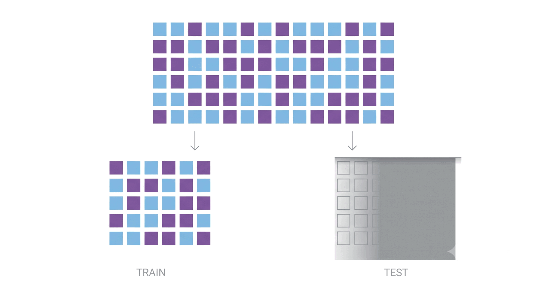
Predictive modelling requires a strict separation between model development and model evaluation. We therefore withhold a subset of caudate samples before any model fitting or tuning.

3.1 Reproduce the published random split

The random seed is taken directly from the authors’ script. Fixing the seed reproduces the same partition and ensures that all participants obtain the same training and test sets.

set.seed(1710)

The split assigns 52 caudate samples to model development and withholds 23 for final evaluation. These 23 samples must remain untouched until the classifier and all tuning choices have been finalized.

d <- counts[, cau]
y <- factor(meta$Diagnosis[cau], levels = c("CTRL", "PD"))

nTest <- ceiling(ncol(d) * 0.3)
ind   <- sample(ncol(d), nTest, FALSE)
c(train = ncol(d) - nTest, test = nTest)

## train  test 
##    52    23

3.2 Construct the MLSeq input objects

Two implementation details follow the authors’ script:
- + 1 adds a pseudocount before normalization. This prevents zeros from invalidating gene-wise geometric means used during size-factor estimation.
- DESeqDataSet is used as the data container expected by MLSeq::classify(). This does not imply that a DESeq2 differential-expression analysis is being performed.

train <- DESeq2::DESeqDataSetFromMatrix(d[, -ind] + 1, S4Vectors::DataFrame(condition = y[-ind]), ~ condition)
test  <- DESeq2::DESeqDataSetFromMatrix(d[,  ind] + 1, S4Vectors::DataFrame(condition = y[ ind]), ~ condition)

4 Step 3 — Tune and train the classifier

4.1 Tune the shrinkage threshold by repeated cross-validation

The control object defines the tuning procedure:
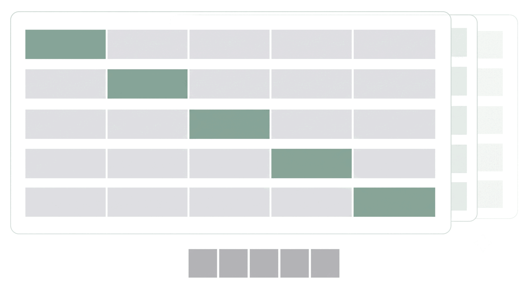
- number = 5 requests five-fold cross-validation: the training set is partitioned into five folds, four are used for fitting, and the remaining fold is used for validation.
- repeats = 10 repeats this process ten times with different fold assignments, reducing sensitivity to a favourable or unfavourable partition.
- tuneLength = 10 evaluates ten candidate shrinkage thresholds.
In total, the tuning procedure fits 5 × 10 × 10 = 500 models before selecting the final threshold.

Cross-validation is performed entirely within the 52-sample training set. The 23 held-out samples do not influence model selection. Once a test set affects tuning, feature selection, or any other analytical choice, it can no longer provide an unbiased estimate of predictive performance.

ctrl <- MLSeq::voomControl(method = "repeatedcv", number = 5, repeats = 10, tuneLength = 10)
fit <- MLSeq::classify(data = train, method = "voomNSC", normalize = "deseq", ref = "CTRL", control = ctrl)

If model fitting is too slow or does not complete, load the precomputed object generated with the same code:

# Note: Load the precomputed object if MLSeq::classify() did not complete
fit <- readRDS("precomputed/classifier_voomNSC_CAU.rds")

5 Step 4 — Identify the predictive gene signature

The fitted classifier retains 19 genes from the original 25,118. All remaining genes are shrunk to zero class difference and therefore do not contribute to prediction.

genes <- MLSeq::selectedGenes(fit)
length(genes)

## [1] 19

The selected set is identical to the 19 genes shown in Figure 1g of the paper.
Several genes have plausible biological interpretations. VGF encodes a neurosecretory protein associated with neurodegenerative processes, whereas TUBB3 is enriched in neurons. The presence of the haemoglobin genes HBA1, HBA2, and HBB requires more cautious interpretation: they may reflect vascular or blood-derived signal, technical variation, or systematic differences in tissue collection. A predictive model can exploit any reproducible association, regardless of whether it is mechanistically related to disease.
This result also illustrates the distinction between differential expression and prediction. Session 4 identified approximately 5,500 genes that differed on average between groups; the classifier retains only 19 because many differentially expressed genes provide redundant predictive information.

sort(genes)

##  [1] "ANGPT2"    "ANGPTL4"   "ANKRD20A2" "CIRBP"     "DEPP1"     "GPCPD1"   
##  [7] "HBA1"      "HBA2"      "HBB"       "LBH"       "LINC01338" "MT1M"     
## [13] "MYBPC1"    "NUPR1"     "SEMA3G"    "TARBP1"    "TRIP10"    "TUBB3"    
## [19] "VGF"

6 Step 5 — Evaluate performance in held-out caudate samples

6.1 Generate predictions for the untouched test set

The 23 held-out caudate samples are evaluated only after model fitting and tuning are complete.

pred <- MLSeq::predictClassify(fit, test)
table(predicted = pred, actual = y[ind])

##          actual
## predicted CTRL PD
##      CTRL   10  1
##      PD      1 11

6.2 Interpret the confusion matrix and accuracy

The confusion matrix shows 21 correct classifications among 23 samples: one PD donor is classified as control, and one control donor is classified as PD.
- Sensitivity: 11/12 = 92%; the classifier identifies 11 of the 12 PD samples.
- Specificity: 10/11 = 91%; the classifier correctly identifies 10 of the 11 control samples.
Accuracy should always be interpreted alongside the class distribution and confusion matrix. In a severely imbalanced dataset, a classifier that predicts only the majority class can achieve high accuracy while providing no useful discrimination. The present test set is approximately balanced, so accuracy is informative, but sensitivity and specificity remain essential.
The paper reports 86% caudate test accuracy, whereas this rerun obtains 91%. With only 23 test samples, one classification changes the reported accuracy by approximately 4.3 percentage points; the difference should therefore not be over-interpreted.

mean(pred == y[ind])

## [1] 0.9130435

7 Step 6 — Evaluate cross-region transfer to the putamen

7.1 Apply the caudate-trained model to an independent brain region

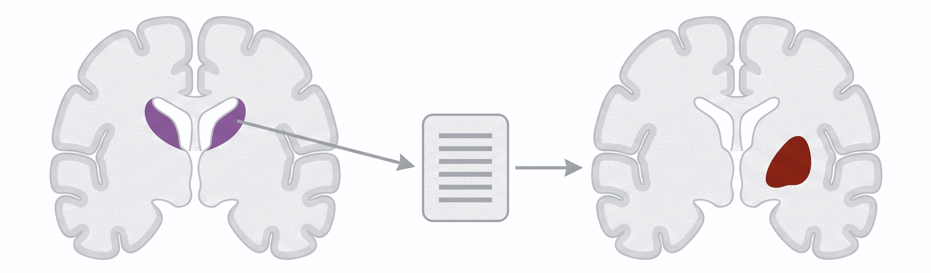
The model was trained on 52 caudate samples and then applied, without retraining, to 75 putamen samples. It correctly classifies approximately 89% of them.
This reproduces the central cross-region result: a signature developed in the caudate retains predictive value in the putamen, suggesting that it captures a disease-associated signal shared across striatal regions.

put_dds <- DESeq2::DESeqDataSetFromMatrix(
               counts[, put] + 1,
               S4Vectors::DataFrame(condition = factor(meta$Diagnosis[put], levels = c("CTRL","PD"))), ~ condition)

pred_put <- MLSeq::predictClassify(fit, put_dds)
mean(pred_put == meta$Diagnosis[put])

## [1] 0.8933333

8 Step 7 — Figure 1g - visualize the 19-gene classifier signature

8.1 Prepare log-CPM expression values and sample annotations

Figure 1g displays log₂ counts per million for the 19 selected genes, standardized separately for each gene across control and PD striatal samples.
The first annotation track uses four colours because it represents the combination of region and diagnosis. A second track displays diagnosis alone, allowing the four experimental groups and the broader disease contrast to be read simultaneously. The palette is retained from Session 4.

lcpm <- edgeR::cpm(counts, log = TRUE)
mat  <- lcpm[genes, ]

8.2 Reproduce the published heatmap design

Two display choices follow the paper rather than the defaults in pheatmap:
- The colour ramp is red–yellow–blue.
- The scale is fixed from -3 to +3 standard deviations, ensuring that colour has the same interpretation across the entire figure.
scale = "row" standardizes each gene to mean 0 and standard deviation 1. This prevents highly expressed haemoglobin genes from dominating the display and emphasizes relative expression patterns across samples, although absolute expression differences between genes are no longer represented.
cluster_cols = FALSE preserves the specified sample order—control before PD and caudate before putamen—so the group-level block structure remains visible. Column clustering would answer a different, unsupervised question.
The resulting heatmap shows a consistent diagnostic pattern in both regions, supporting the transferability of the selected signature.

PAL4 <- c(CTRL_CAU = "#7FBEE7", CTRL_PUT = "#ECAC1F",
          PD_CAU   = "#7F509F", PD_PUT   = "#8A271B")

lab <- c(CTRL_CAU = "Control Caudate", CTRL_PUT = "Control Putamen",
         PD_CAU   = "PD Caudate",      PD_PUT   = "PD Putamen")

ann <- data.frame(
  Region    = factor(lab[as.character(meta$group)], levels = lab),
  Diagnosis = factor(ifelse(meta$Diagnosis == "CTRL", "Control", "PD"),
                     levels = c("Control", "PD")))
rownames(ann) <- meta$Sample

ann_col <- list(
  Region    = setNames(unname(PAL4[names(lab)]), lab),
  Diagnosis = c(Control = "#93C73D", PD = "#2A4EA0"))

ord <- order(meta$Diagnosis, meta$Region)

pheatmap::pheatmap(mat[, ord],
         annotation_col    = ann,
         annotation_colors = ann_col,
         cluster_cols      = FALSE,
         scale             = "row",
         show_colnames     = FALSE,
         fontsize_row      = 8,
         color  = colorRampPalette(rev(RColorBrewer::brewer.pal(11, "RdYlBu")))(100),
         breaks = seq(-3, 3, length.out = 101))

9 Step 8 — Compare our results with the published analysis

Quantity	Ours	Paper
Classifier genes	19	19
The gene list	identical	identical
Caudate test accuracy	91.3%	86%
Putamen accuracy	89.3%	90%

The reproduced classifier contains exactly the same 19 genes as the published model.
This close agreement is supported by three features of the workflow:
- The authors released the original random seed, set.seed(1710), allowing the same 52/23 partition to be reconstructed.
- Once the split and tuning procedure are fixed, nearest shrunken centroids does not depend on a random model initialization.
- Changes in MLSeq versions have not materially altered the fitted signature in this analysis.
This differs from Session 4, where exact reproduction was prevented by an unavailable death-age covariate. Reproducibility depends not only on code availability but also on access to every variable used in the original model.

9.1 Sensitivity analysis — Change the random split

Change the random seed and rerun the analysis from Step 2. A new seed creates a different training/test split and may change the selected genes and estimated accuracy.
With only 75 caudate samples, the 19-gene signature should not be treated as an immutable biological set. It is one model derived from one partition of the cohort. Genes that recur across many resampled splits provide stronger evidence of selection stability than genes that appear only once.
Repeating the workflow across seeds is therefore a simple sensitivity analysis for both feature stability and performance variability.

set.seed(2024)

10 Session summary and key takeaways

A held-out test set provides the most defensible estimate of performance on unseen data. Training-set or cross-validation performance alone is not a final evaluation.
Hyperparameter tuning and feature selection must occur entirely within the training data. Any use of the test set during model development compromises its independence.
Differential expression and classification answer different questions: thousands of genes may differ between groups, while a much smaller subset may be sufficient for prediction.
External or transfer validation is more informative than evaluation in the same data domain. Applying the caudate-trained model to the putamen tests whether the signature generalizes across brain regions.
Predictive features require biological and technical scrutiny. The haemoglobin genes may contribute useful signal, but they also raise questions about tissue composition, sample handling, and potential confounding.

HUB (Hands-on Understanding of Bioinformatics) Workshop Bulk RNA-seq Data Analysis by Bioinformatics Hub

[Session 5] From Expression Signatures to Prediction: Building and Evaluating a Sample Classifier

1 Introduction

1.1 Study overview and prediction task

1.2 Published workflow and analytical approach

1.3 How the voomNSC classifier works

1.4 Environment

2 Step 1 — Load the data and define the regional cohorts

2.1 Load and validate the count matrix and metadata

2.2 Define the caudate training cohort and putamen transfer cohort

3 Step 2 — Create independent training and test sets

3.1 Reproduce the published random split

3.2 Construct the MLSeq input objects

4 Step 3 — Tune and train the classifier

4.1 Tune the shrinkage threshold by repeated cross-validation

5 Step 4 — Identify the predictive gene signature

6 Step 5 — Evaluate performance in held-out caudate samples

6.1 Generate predictions for the untouched test set

6.2 Interpret the confusion matrix and accuracy

7 Step 6 — Evaluate cross-region transfer to the putamen

7.1 Apply the caudate-trained model to an independent brain region

8 Step 7 — Figure 1g - visualize the 19-gene classifier signature

8.1 Prepare log-CPM expression values and sample annotations

8.2 Reproduce the published heatmap design

9 Step 8 — Compare our results with the published analysis

9.1 Sensitivity analysis — Change the random split

10 Session summary and key takeaways

HUB (Hands-on Understanding of Bioinformatics) Workshop
Bulk RNA-seq Data Analysis
by Bioinformatics Hub

[Session 5] From Expression Signatures to Prediction:
Building and Evaluating a Sample Classifier