[Session 3] From FASTQ Files to Gene Counts:
Alignment and Quantification.

1 Introduction

1.1 Session overview

This is Session 3 of the HUB Workshop Series 3 (Bulk RNA-seq), covering how sequencing reads (FASTQ) are turned into a gene × sample count table — the object the afternoon sessions start from.
Two independent routes are run on the same reads and then compared:
- Alignment-based (STAR): map reads to the genome, then count reads per gene.
- Alignment-free (Salmon): map reads directly to transcripts, then roll up to genes.
The focus is the mechanics of alignment and quantification, not biological interpretation.

1.2 Learning objectives

Run an alignment-based pipeline with STAR: build an index, align two samples, and produce per-gene counts.
Run an alignment-free pipeline with Salmon: build a transcript index, quantify, and roll up transcripts to genes.
Compare the two gene-level count tables and understand where, and why, they disagree.

1.3 Workshop materials and data

Everything runs inside the thebiohub/bulkrnaseq Docker container on your own laptop.
The curated workshop materials are available for download here: BulkRNAseq.zip (295.5 MB)

2 Environment

To support reproducible research, the whole session runs inside a Docker-based analysis environment.
Software (bundled in the image):
- STAR (v2.7.11b)
- salmon (v1.10.3)
- samtools (v1.21)
- gffread (v0.12.9)

3 Step 0 — Start the workshop environment

3.1 Download the Docker image

Do this once, before the workshop — it is a ~2 GB download.

docker pull --platform linux/amd64 thebiohub/bulkrnaseq

3.2 Launch the container and mount the workshop directory

Run this in Terminal (macOS/Linux)

docker run -it -v ~/Desktop/BulkRNAseq:/workshop/data thebiohub/bulkrnaseq bash

Run this in or PowerShell (Windows)

docker run -it -v ${HOME}\Desktop\BulkRNAseq:/workshop/data thebiohub/bulkrnaseq bash

3.3 Verify the mounted files

Everything from here on is typed inside the container. Check the mount worked:

pwd
ls
tree -L 2 data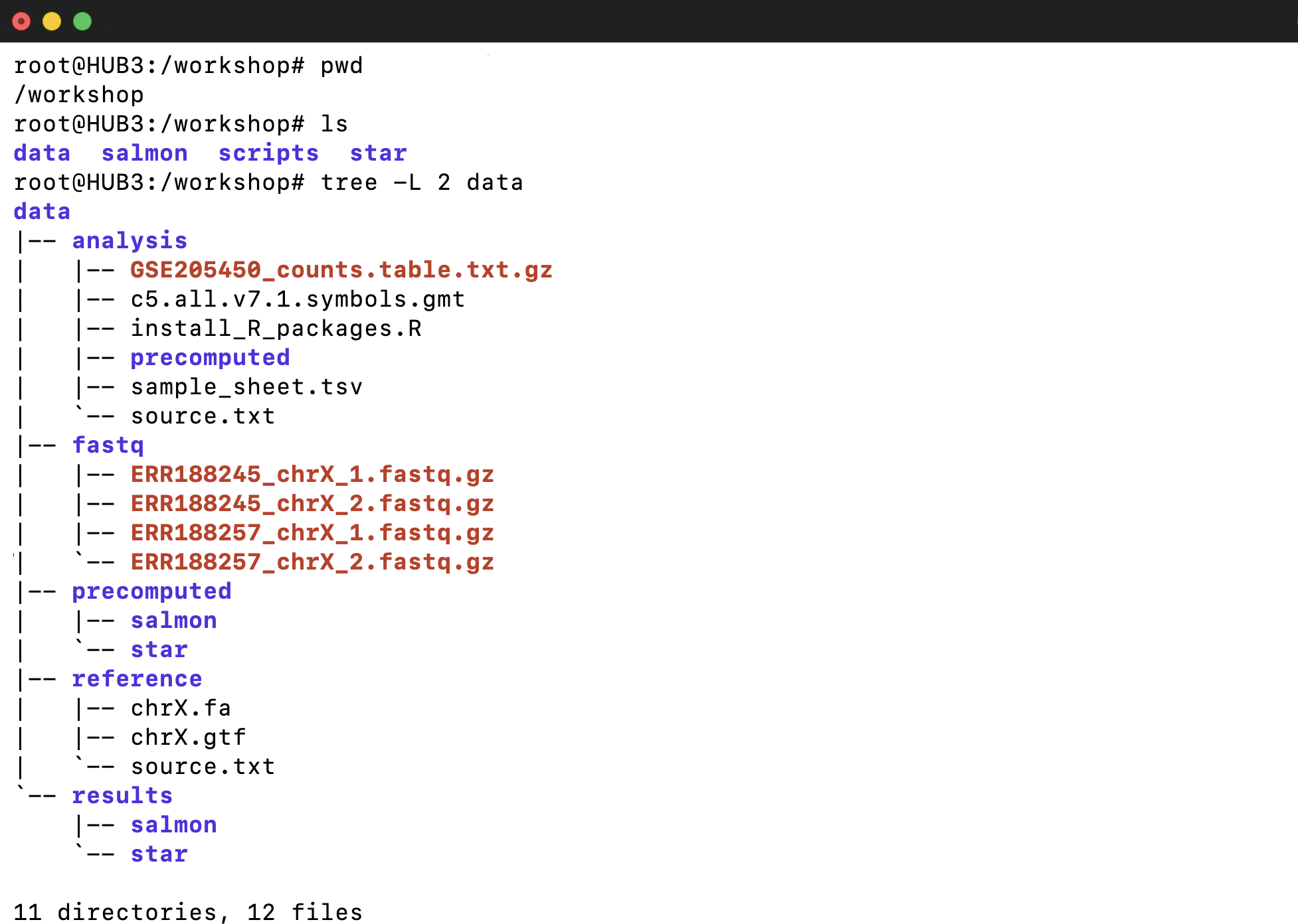

4 Pipeline A — Genome alignment and gene counting with STAR

STAR (Spliced Transcripts Alignment to a Reference), Dobin et al. Bioinformatics (2013)
Align reads to the genome, then count reads per gene. A complete, self-contained pipeline: Steps A.1 through A.9.

4.1 Confirm the required software

Before we build anything, let’s make sure the two tools we’ll rely on are installed, and note their versions for reference.

STAR --version
samtools --version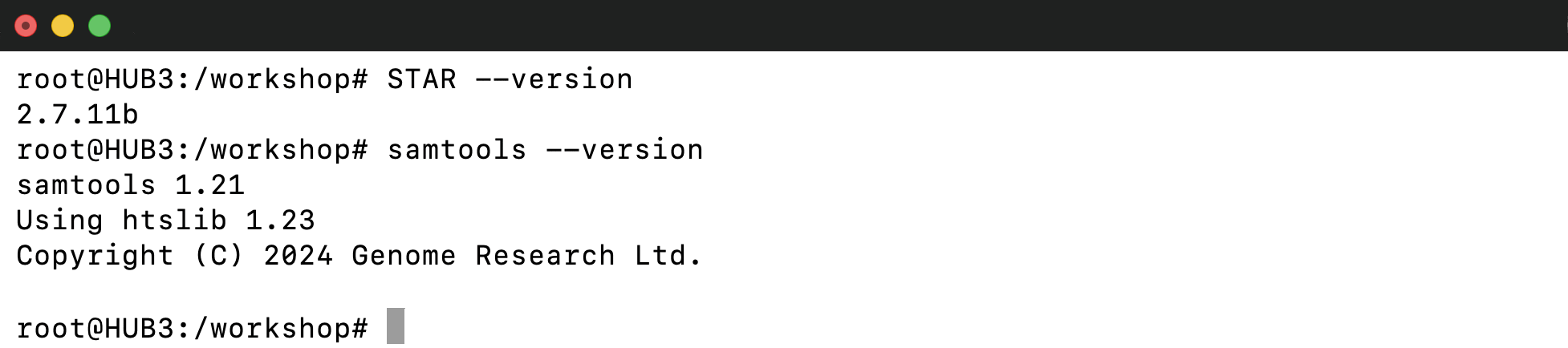

4.2 Inspect the input FASTQ files

A quick look to confirm the two paired-end samples are where we expect them, before we point STAR at them.

ls data/fastq

4.3 Build the STAR genome index

STAR does not read raw FASTA at alignment time — it first turns the genome and annotation into a fast, searchable index. We build that index once here, and every alignment step below reuses it.
You don’t need to type the entire path manually—use Tab completion to save time. For example, type wo and press ‘Tab’ to autocomplete the path.
--genomeSAindexNbases sets the length of the seed lookup table in STAR’s genome index. Set it to 12 for the workshop to reduce runtime and memory usage; the default of 14 is designed for whole-genome data.
No worries if this ends in “Killed” — that just means your laptop ran out of memory while building the index. Use the fallback below and copy the prebuilt one; the rest of the workshop is identical.

mkdir -p /workshop/data/results/star/index

STAR --runMode genomeGenerate \
     --runThreadN 2 \
     --genomeDir /workshop/data/results/star/index \
     --genomeFastaFiles /workshop/data/reference/chrX.fa \
     --sjdbGTFfile /workshop/data/reference/chrX.gtf \
     --sjdbOverhang 75 \
     --genomeSAindexNbases 12

ls /workshop/data/results/star/index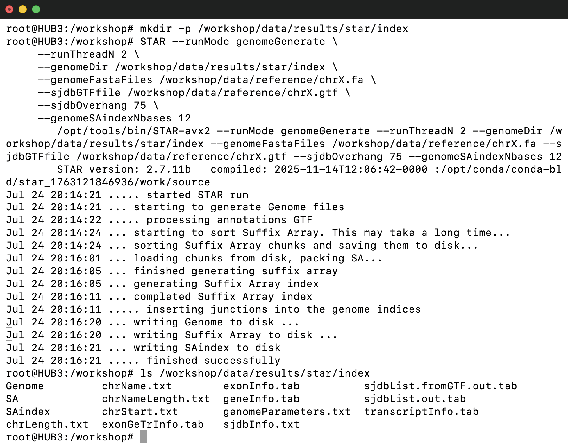

Fallback — copy out the prebuilt STAR index. If index generation fails on your machine, copy the prebuilt index we prepared in advance and continue:

# Note: This is a fallback step and is only needed if the STAR index generation fails.
cp -rf /workshop/star/index/. /workshop/data/results/star/index/
ls /workshop/data/results/star/index

4.4 Align the first sample to the genome

Now the main event: STAR places each read pair on the genome, and — thanks to --quantMode GeneCounts — tallies reads per gene in the same pass.

STAR --runThreadN 2 \
     --genomeDir /workshop/data/results/star/index \
     --readFilesIn /workshop/data/fastq/ERR188245_chrX_1.fastq.gz \
                   /workshop/data/fastq/ERR188245_chrX_2.fastq.gz \
     --readFilesCommand zcat \
     --outSAMtype BAM SortedByCoordinate \
     --quantMode GeneCounts \
     --outFileNamePrefix /workshop/data/results/star/ERR188245_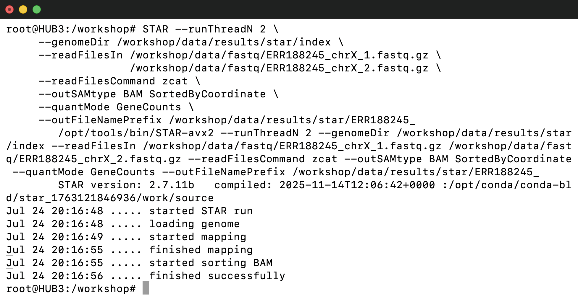

4.5 Align the second sample to the genome

The very same command for the second sample — only the input FASTQs and the output prefix change. In a real study you would wrap this in a loop over all samples.

STAR --runThreadN 2 \
     --genomeDir /workshop/data/results/star/index \
     --readFilesIn /workshop/data/fastq/ERR188257_chrX_1.fastq.gz \
                   /workshop/data/fastq/ERR188257_chrX_2.fastq.gz \
     --readFilesCommand zcat \
     --outSAMtype BAM SortedByCoordinate \
     --quantMode GeneCounts \
     --outFileNamePrefix /workshop/data/results/star/ERR188257_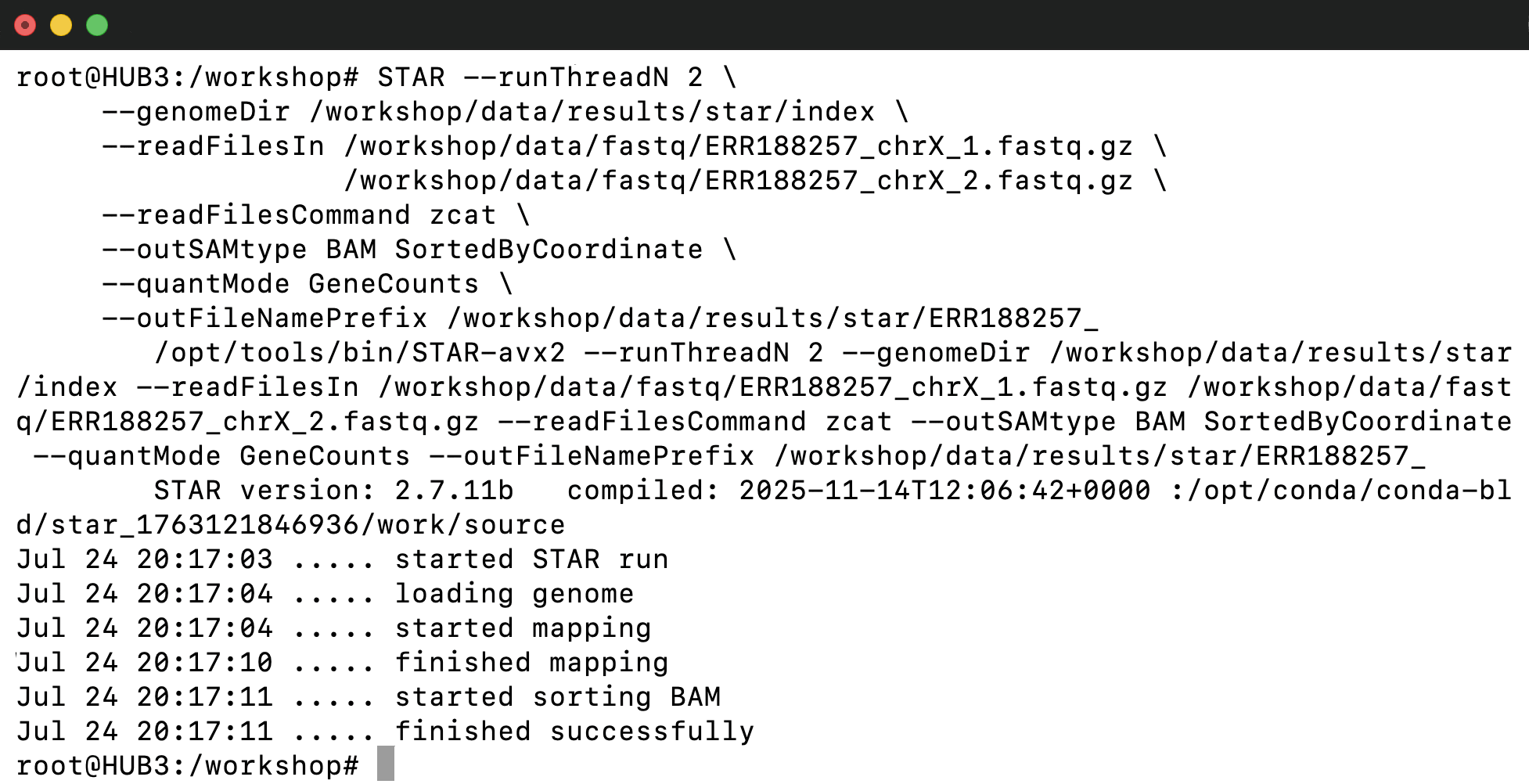

4.6 Evaluate STAR alignment quality

Log.final.out is STAR’s own summary of how the run went.

cat /workshop/data/results/star/ERR188245_Log.final.out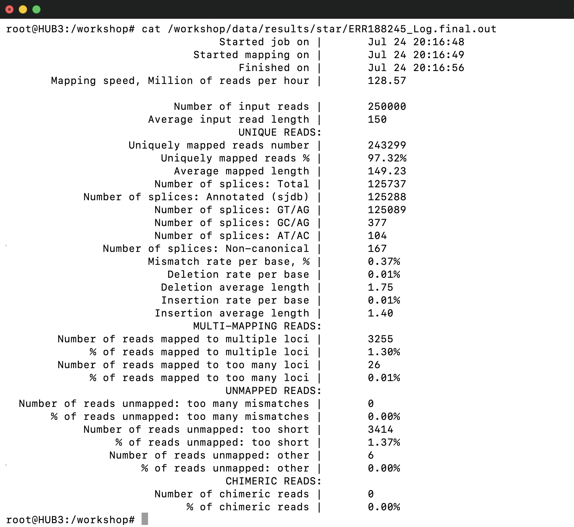

The uniquely-mapped rate is the first thing worth checking — it tells us how cleanly the reads landed on the genome.

grep "Uniquely mapped reads %" /workshop/data/results/star/ERR188245_Log.final.out
grep "Uniquely mapped reads %" /workshop/data/results/star/ERR188257_Log.final.out

4.7 Inspect the per-gene count output

Column 1 is the gene, column 2 the unstranded count, columns 3 and 4 the two stranded options.

head /workshop/data/results/star/ERR188245_ReadsPerGene.out.tab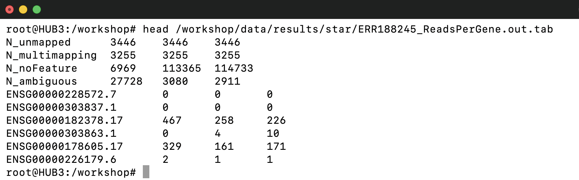

The first 4 rows are summary rows, so skip them to count how many genes actually picked up a read.

tail -n +5 /workshop/data/results/star/ERR188245_ReadsPerGene.out.tab | awk '$2 > 0' | wc -l
tail -n +5 /workshop/data/results/star/ERR188245_ReadsPerGene.out.tab | wc -l

4.8 Inspect genomic alignments with samtools

Index the BAM first — the .bai lets tview and region queries jump straight to a position instead of scanning the whole file.

samtools index /workshop/data/results/star/ERR188245_Aligned.sortedByCoord.out.bam
ls /workshop/data/results/star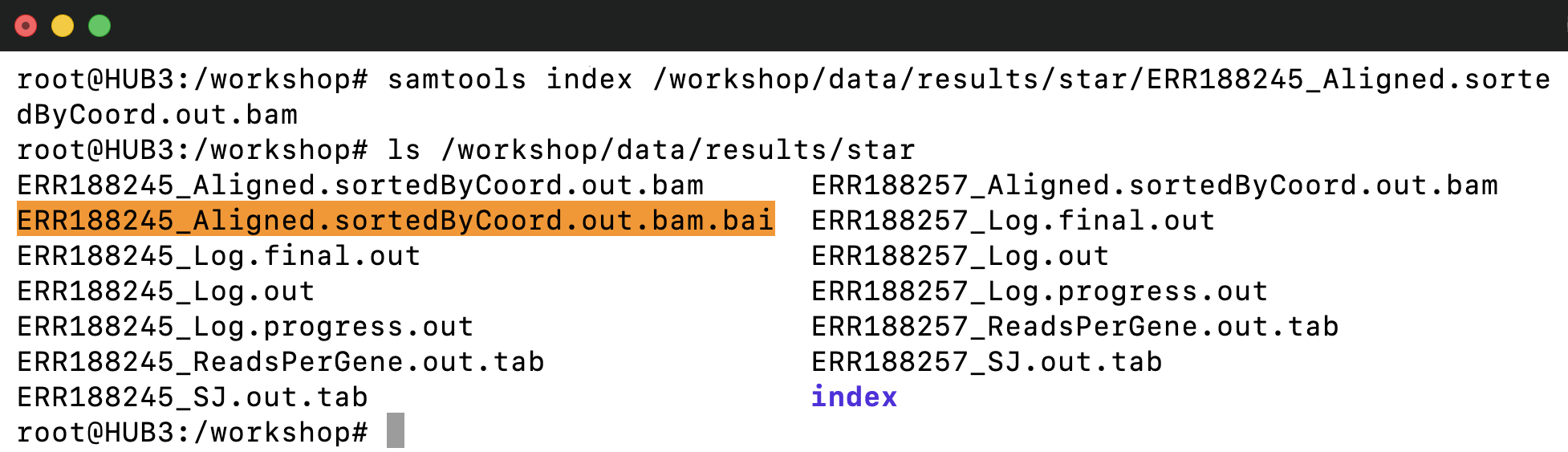

Next, inspect the BAM by viewing its header, a few alignment records, and a summary of the alignment statistics.

samtools view -H /workshop/data/results/star/ERR188245_Aligned.sortedByCoord.out.bam
samtools view /workshop/data/results/star/ERR188245_Aligned.sortedByCoord.out.bam | head -3
samtools flagstat /workshop/data/results/star/ERR188245_Aligned.sortedByCoord.out.bam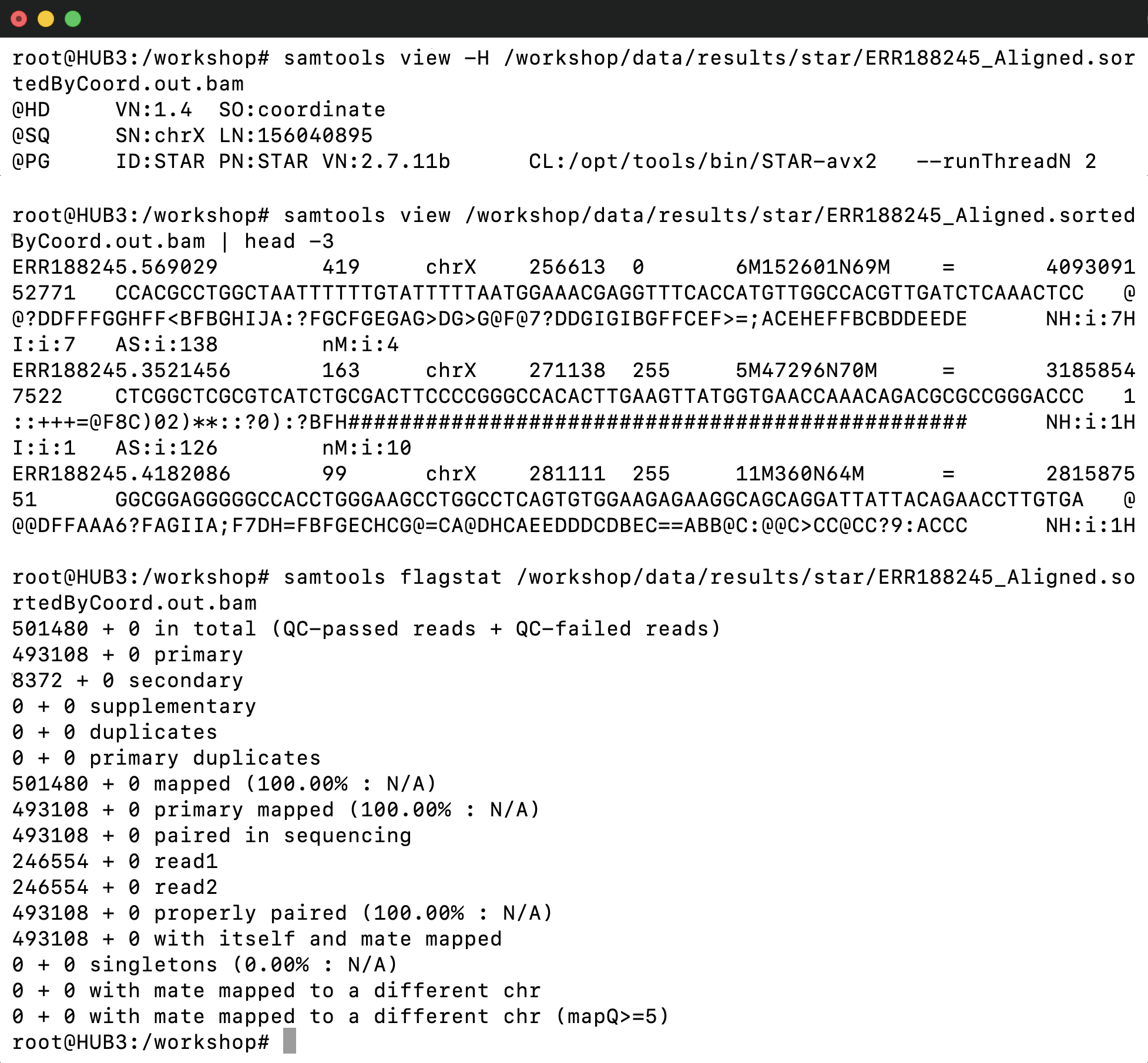

Finally, open the alignments in a terminal-based viewer to explore how the reads align to the reference sequence.

samtools tview /workshop/data/results/star/ERR188245_Aligned.sortedByCoord.out.bam /workshop/data/reference/chrX.fa

Inside tview:

g                    go to region
chrX:73820651
n                    color by nucleotide  (A green, C cyan, G magenta, T red, N blue)
b                    color by base quality (>=30 white, 20-29 yellow, 10-19 green, 0-9 blue)
m                    color by mapping quality (>=30 white, 20-29 yellow, 10-19 green, 0-9 blue)
q                    quit / leave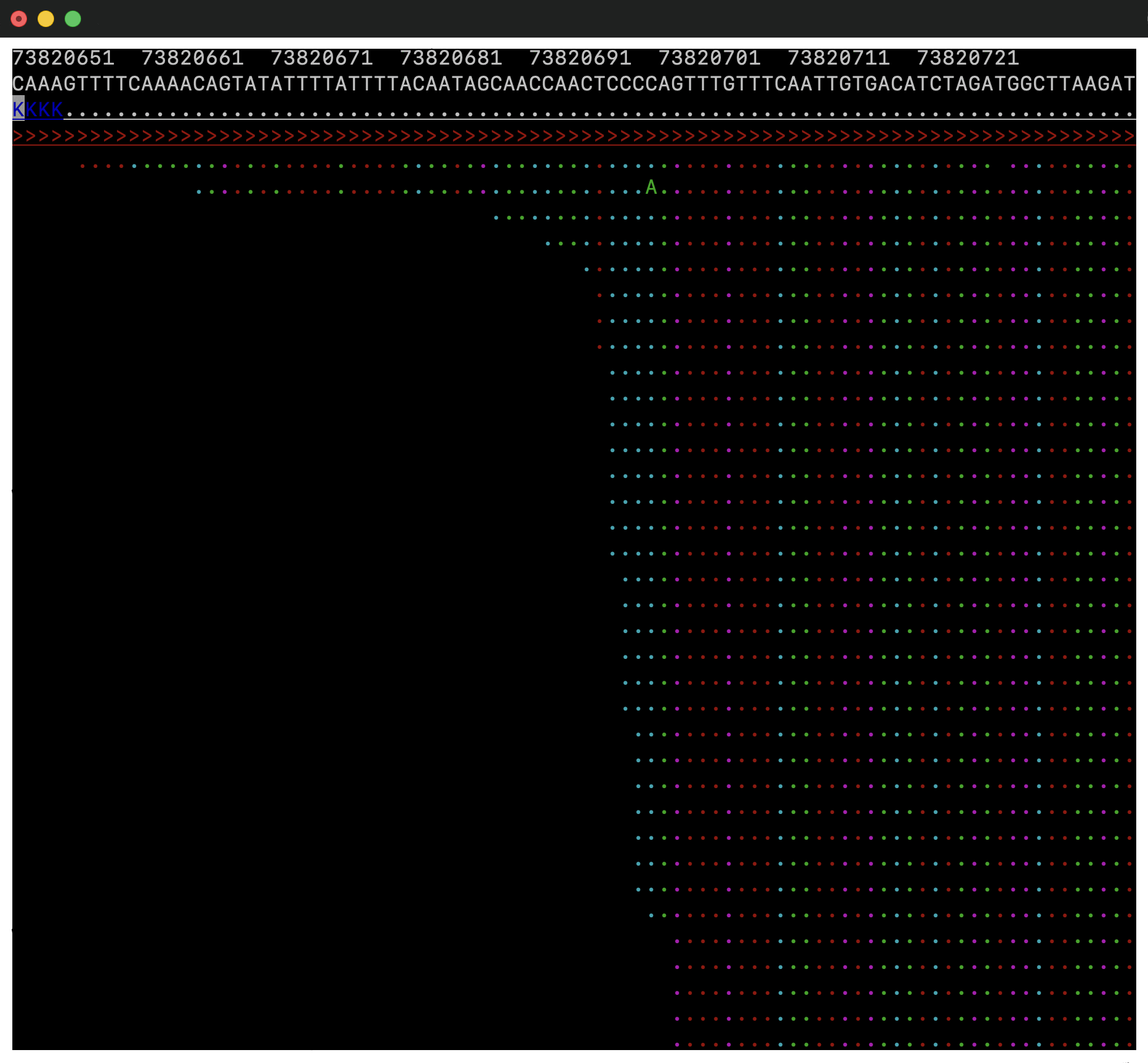

4.9 Assemble the STAR gene-count matrix

First, create an output file containing the column names (gene_id and one column for each sample).

printf "gene_id\tERR188245\tERR188257\n" > /workshop/data/results/star/gene_counts.tsv
cat /workshop/data/results/star/gene_counts.tsv

Concatenate the two per-gene files (from the two alignment steps) into one gene × sample matrix. Minimum columns: gene_id plus one count column per sample.

paste <(tail -n +5 /workshop/data/results/star/ERR188245_ReadsPerGene.out.tab | cut -f1,2) \
      <(tail -n +5 /workshop/data/results/star/ERR188257_ReadsPerGene.out.tab | cut -f2) \
      >> /workshop/data/results/star/gene_counts.tsv
head /workshop/data/results/star/gene_counts.tsv
wc -l /workshop/data/results/star/gene_counts.tsv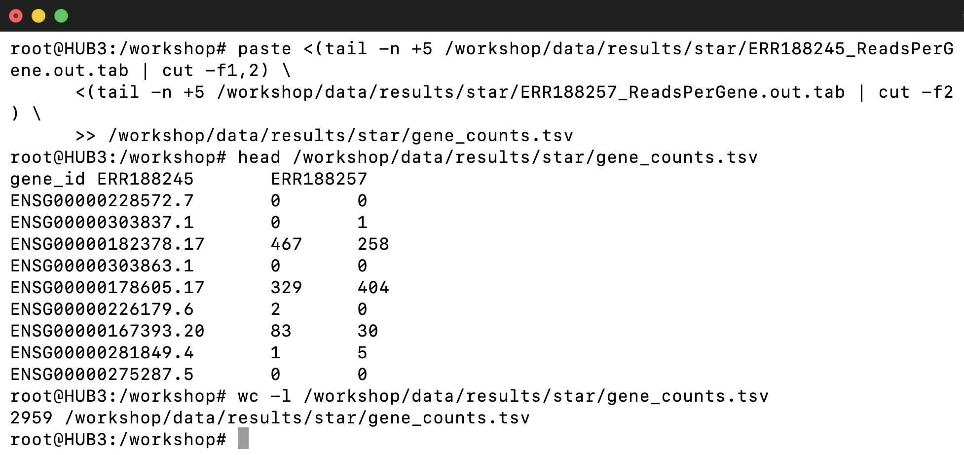

5 Pipeline B — Transcript quantification with Salmon

A completely separate pipeline. Salmon does not use the genome, the STAR index, or the BAMs from Pipeline A — it maps reads directly to transcripts. You can run Pipeline B without having run Pipeline A at all.

5.1 Confirm the required software

Same idea as in Pipeline A, now for Salmon and gffread — a quick check that both are on hand before we start.

salmon --version
gffread --version

5.2 Build the transcriptome FASTA

Salmon maps to transcripts, so it needs a transcript FASTA. You build it from the two downloaded reference files — the genome (chrX.fa) and the annotation (chrX.gtf) — the same pair STAR used in Pipeline A.
First look at the annotation. Column 3 of a GTF is the feature type, column 9 the attributes; count how many genes chrX carries:

grep -v "^#" /workshop/data/reference/chrX.gtf | head -3
awk -F'\t' '$3 == "gene"' /workshop/data/reference/chrX.gtf | wc -l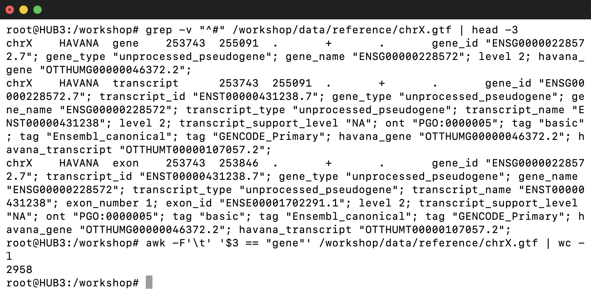

Now extract one spliced sequence per transcript record with gffread:

gffread -w /workshop/data/reference/chrX.transcripts.fa \
        -g /workshop/data/reference/chrX.fa \
        /workshop/data/reference/chrX.gtf

grep -c ">" /workshop/data/reference/chrX.transcripts.fa
head /workshop/data/reference/chrX.transcripts.fa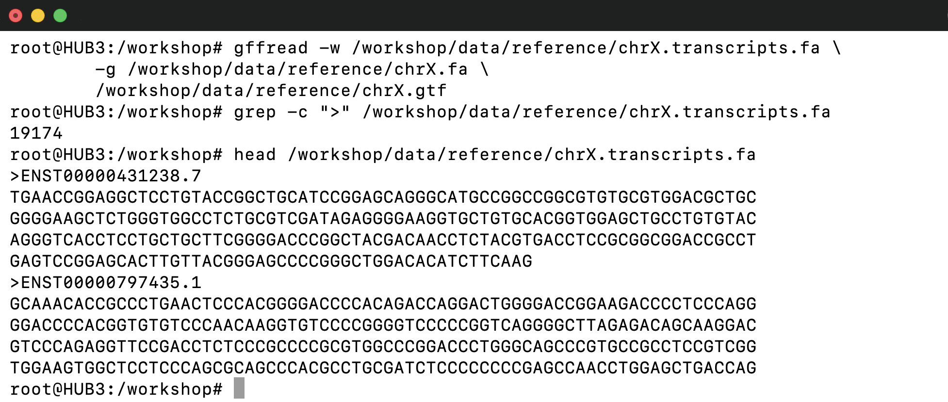

5.3 Build the Salmon transcript index

Build the Salmon index from the transcript FASTA you just made. This is light — it does not need the big STAR memory.

salmon index \
  -p 2 \
  -t /workshop/data/reference/chrX.transcripts.fa \
  -i /workshop/data/results/salmon/index

ls /workshop/data/results/salmon/index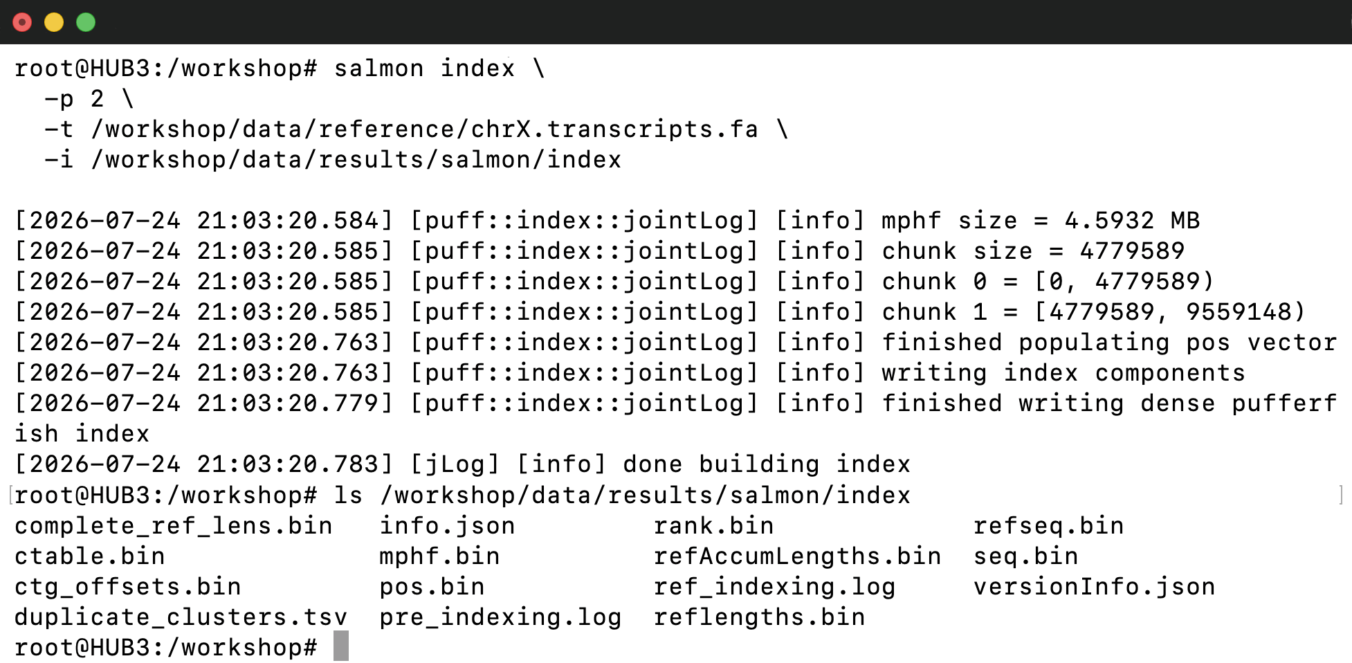

Fallback — copy out the prebuilt Salmon index. If index generation fails, copy the prebuilt index we prepared in advance and continue:

# Note: This is a fallback step and is only needed if the Salmon index generation fails.
cp -rf /workshop/salmon/index/. /workshop/data/results/salmon/index/

5.4 Quantify the first sample with Salmon

Salmon never touches the genome — it assigns reads straight to transcripts.
The -l option specifies the library type (how the reads were prepared and sequenced).
-l A tells Salmon to automatically detect the library type from the input reads, so you don’t need to specify it manually.

salmon quant -i /workshop/data/results/salmon/index \
             -p 2 \
             -l A \
             -1 /workshop/data/fastq/ERR188245_chrX_1.fastq.gz \
             -2 /workshop/data/fastq/ERR188245_chrX_2.fastq.gz \
             -o /workshop/data/results/salmon/ERR188245

head /workshop/data/results/salmon/ERR188245/quant.sf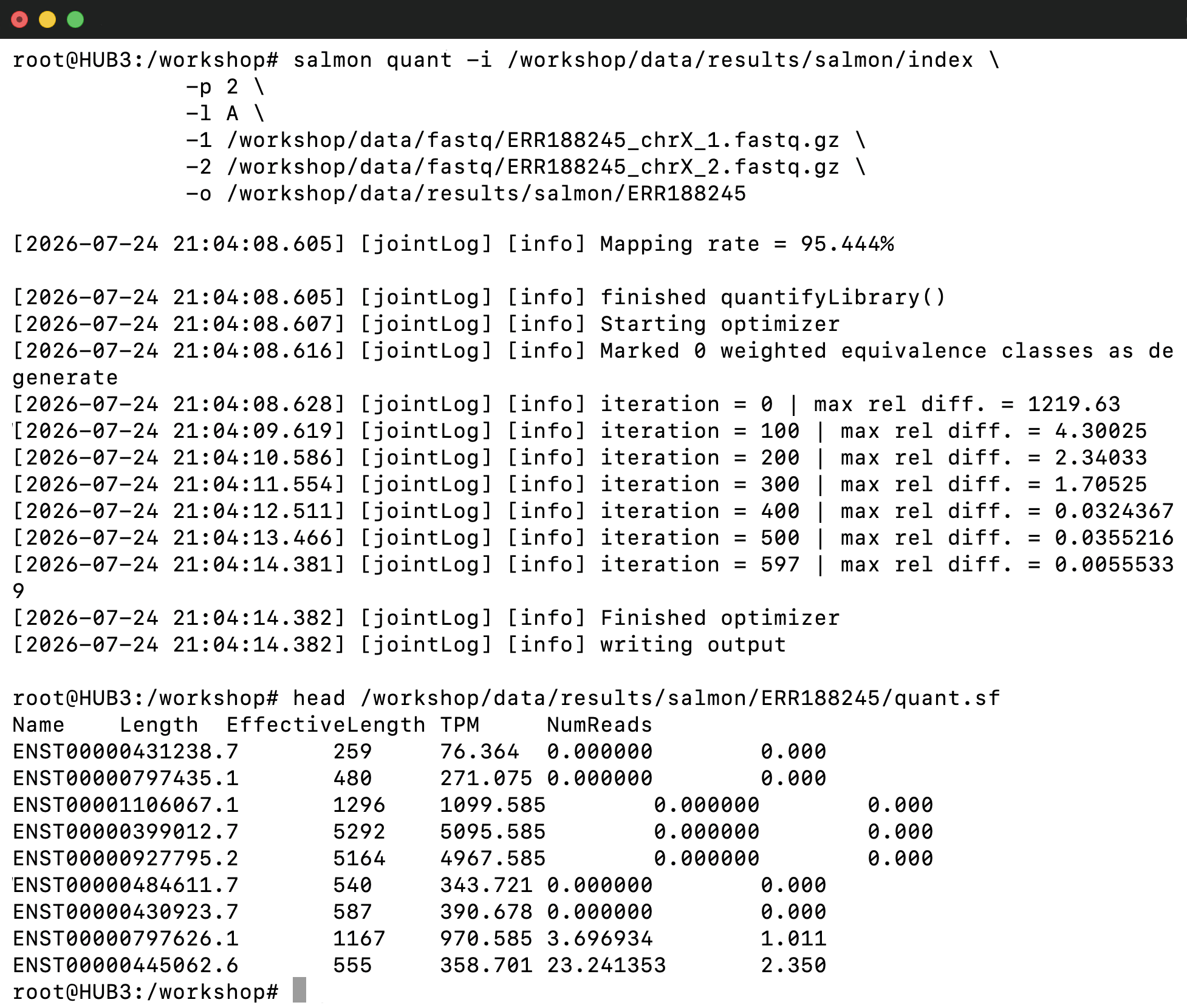

quant.sf columns:

Name             transcript ID
Length           transcript length in bp
EffectiveLength  length adjusted for the fragment-length distribution;
                 this is what converts between counts and TPM
TPM              Transcripts Per Million; relative abundance, sums to
                 1,000,000 across all transcripts
NumReads         estimated reads assigned to the transcript (fractional,
                 because multimapping reads are split probabilistically)

5.5 Quantify the second sample with Salmon

As in Pipeline A, the second sample runs exactly the same way — only the input FASTQs and the output folder change.

salmon quant -i /workshop/data/results/salmon/index \
             -p 2 \
             -l A \
             -1 /workshop/data/fastq/ERR188257_chrX_1.fastq.gz \
             -2 /workshop/data/fastq/ERR188257_chrX_2.fastq.gz \
             -o /workshop/data/results/salmon/ERR188257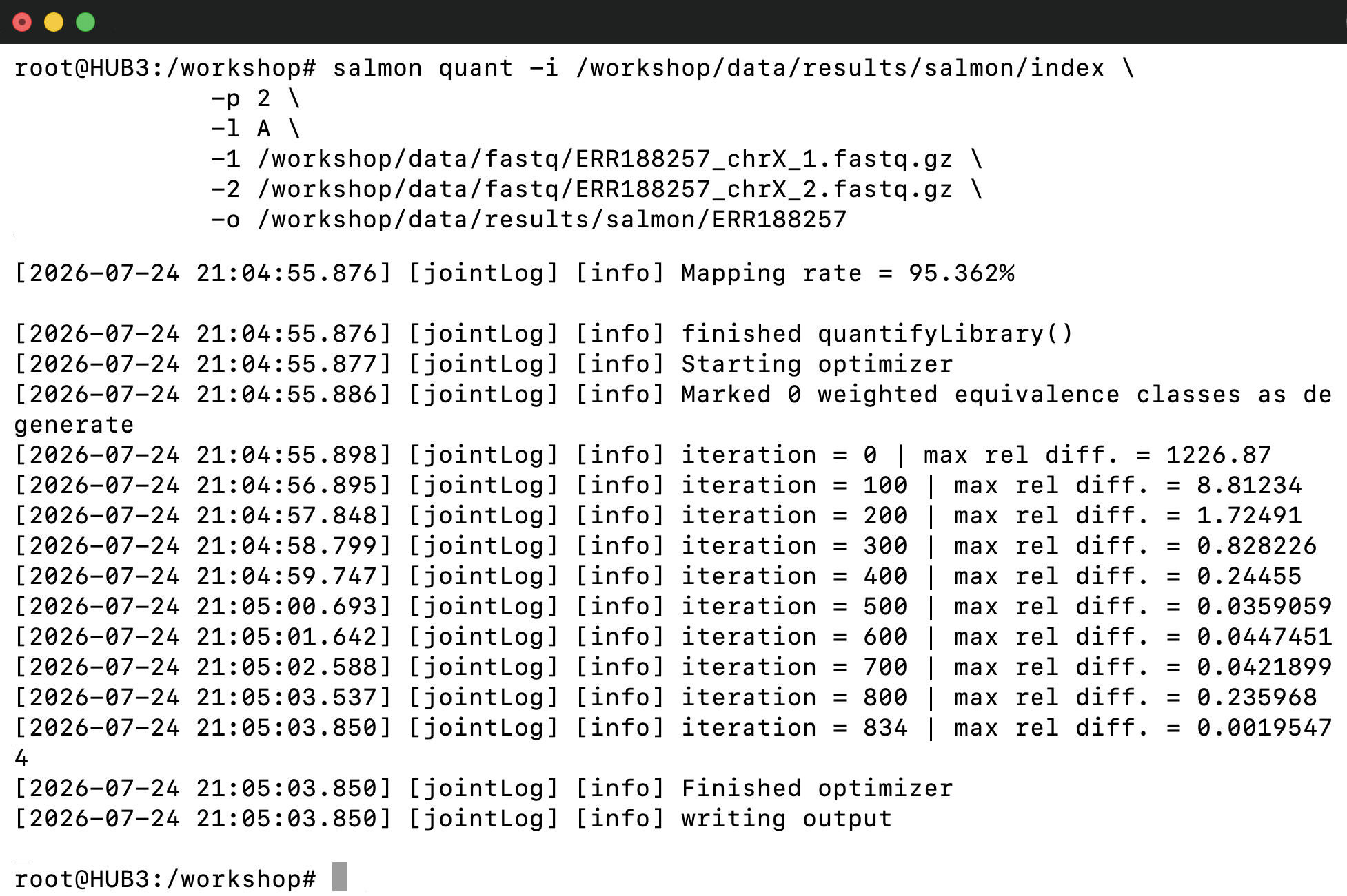

5.6 Evaluate Salmon mapping rates

Salmon records how much of each sample it could assign to transcripts. The mapping rate is the headline number, so let’s pull just that line from each log.

grep -i "Mapping rate" /workshop/data/results/salmon/ERR188245/logs/salmon_quant.log
grep -i "Mapping rate" /workshop/data/results/salmon/ERR188257/logs/salmon_quant.log

5.7 Build the transcript-to-gene mapping table

quant.sf is per transcript; most analyses want per gene. The bridge is a tx2gene map — three columns, TXID GENEID GENESYMBOL — built from the same GTF. gffread’s --table option prints exactly these columns; add the header first:

printf "TXID\tGENEID\tGENESYMBOL\n" > /workshop/data/reference/tx2gene.tsv
cat /workshop/data/reference/tx2gene.tsv

Do not be surprised if GENESYMBOL sometimes repeats the gene ID rather than a readable name: about 3,000 of the 19,174 records have no gene_name in the GTF, and gffread falls back to the ID. Only TXID and GENEID drive the rollup, so this is cosmetic.

gffread /workshop/data/reference/chrX.gtf \
        --table @id,@geneid,gene_name \
        >> /workshop/data/reference/tx2gene.tsv
head /workshop/data/reference/tx2gene.tsv
wc -l /workshop/data/reference/tx2gene.tsv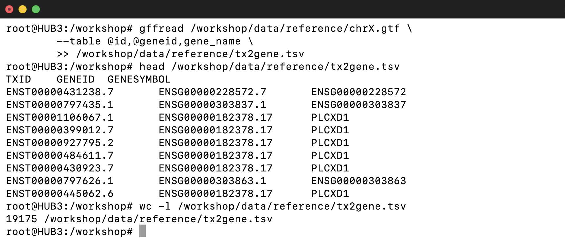

5.8 Summarize transcript estimates to gene-level counts

tximport reads each sample’s quant.sf (per transcript) and sums it to per gene using the tx2gene map, producing one gene × sample count matrix.
This is the gene-level Salmon analog of the STAR gene table: the two pipelines converge here, both yielding a gene × sample matrix — one via STAR --quantMode GeneCounts (integer counts), the other via salmon + tximport (tximport-corrected, fractional counts). Same shape, two independent routes.

more /workshop/scripts/tximport_rollup.R

Rscript /workshop/scripts/tximport_rollup.R
head /workshop/data/results/salmon/gene_counts.tsv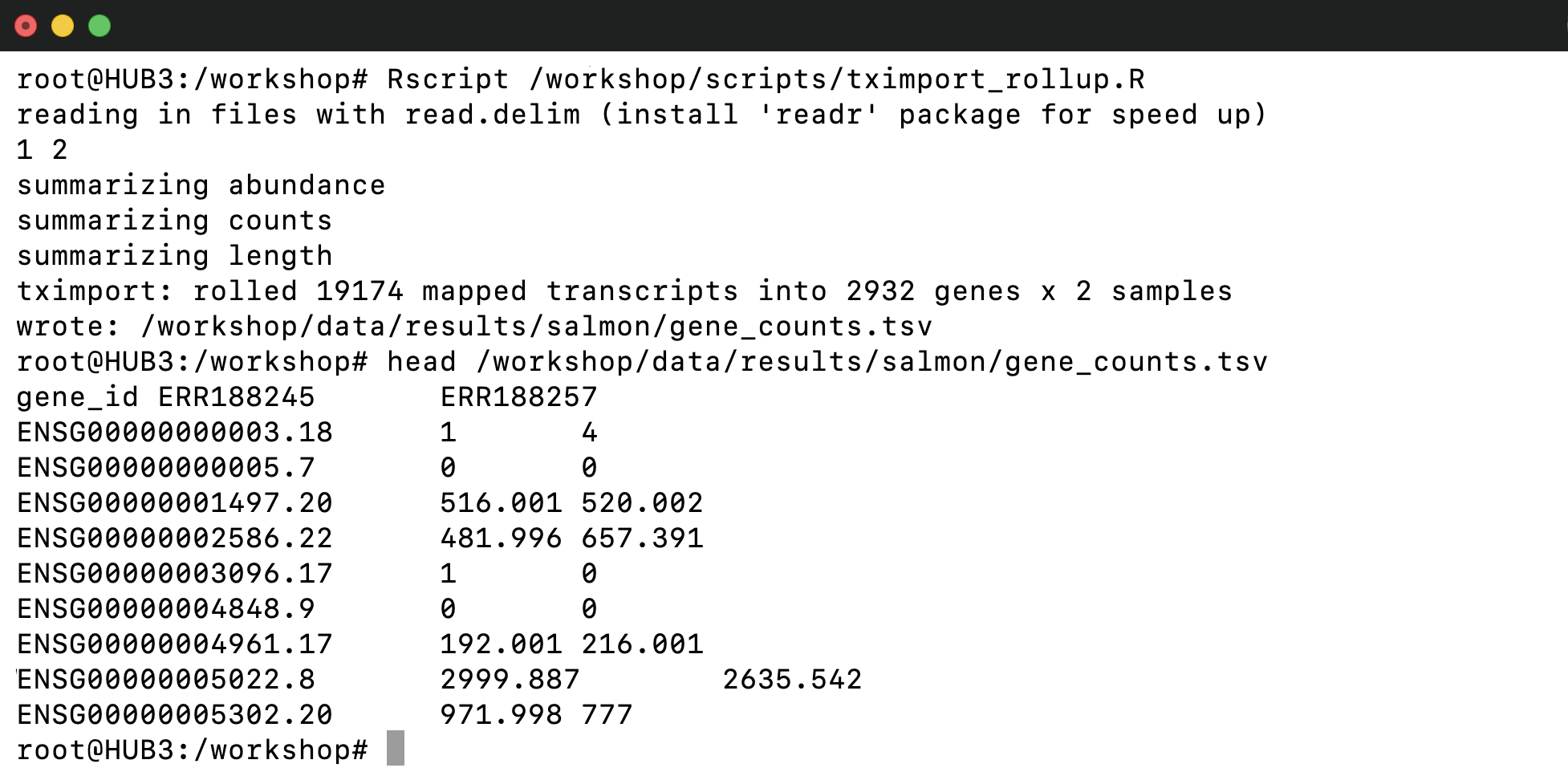

6 Compare gene-level counts from STAR and Salmon

Both pipelines produced a gene × sample count table keyed on the same Ensembl gene_id. Plot one against the other — if they agree, points hug the y = x line. X-axis is STAR, Y-axis is Salmon; each dot is one chrX gene. Counts span orders of magnitude, so transform with asinh — like a log at large counts but defined at zero (asinh(0) = 0), so no pseudocount is needed.
Start R, paste the block, and it writes a PDF to your results folder:

R

star   <- read.delim("/workshop/data/results/star/gene_counts.tsv")
salmon <- read.delim("/workshop/data/results/salmon/gene_counts.tsv")

# keep genes quantified by BOTH pipelines, matched on gene_id
m <- merge(star, salmon, by = "gene_id", suffixes = c(".star", ".salmon"))
cat(nrow(m), "chrX genes shared by both pipelines\n")

pdf("/workshop/data/results/star_vs_salmon.pdf", width = 10, height = 5)
par(mfrow = c(1, 2))
for (s in c("ERR188245", "ERR188257")) {
  x <- asinh(m[[paste0(s, ".star")]])
  y <- asinh(m[[paste0(s, ".salmon")]])
  plot(x, y, pch = 16, cex = 0.6, col = rgb(0, 0, 0, 0.4),
       xlab = paste("STAR  asinh(count)  -", s),
       ylab = paste("Salmon  asinh(count)  -", s))
  abline(0, 1, col = "red")
  legend("topleft", bty = "n", legend = paste("r =", round(cor(x, y), 3)))
}
dev.off()

q("no")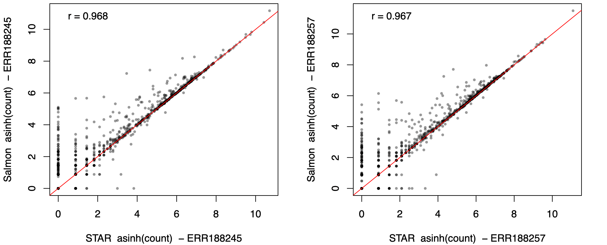

6.1 Match genes quantified by both pipelines

A few dots sit off the y = x line: genes STAR counts as 0 but Salmon does not. A clear case is PABPC1P3, a 458 bp processed pseudogene lying entirely inside the gene RLIM:
About 418 reads, ~392 of them uniquely mapped — good, high-quality reads, not junk. They simply fall inside RLIM as well. STAR’s --quantMode GeneCounts will not count a read that overlaps two genes (it goes to N_ambiguous), so the nested pseudogene gets 0. Salmon maps to transcripts and apportions a share to the pseudogene isoform, so it reports ~82.
Neither is a bug: STAR is conservative about overlaps, Salmon is not. And it is tunable — how multi-mapped reads are treated (dropped, assigned to a single best hit, or split fractionally across the genes or transcripts they match) is a setting you can change in each tool, making either one stricter or more permissive.

RLIM       ENSG00000131263    chrX:74,582,976-74,614,646   (31.7 kb)
PABPC1P3   ENSG00000230673    chrX:74,583,088-74,583,546   (458 bp, nested)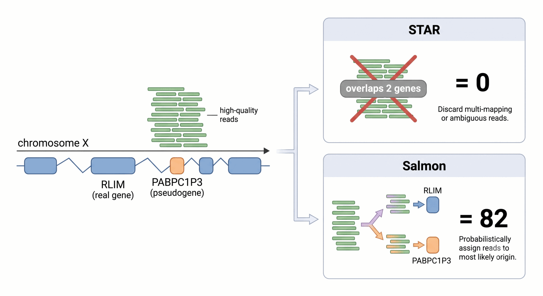

6.2 Compare sample-level count estimates

Compare each pipeline’s count for the two genes:

grep -E "ENSG00000131263|ENSG00000230673" /workshop/data/results/star/gene_counts.tsv
grep -E "ENSG00000131263|ENSG00000230673" /workshop/data/results/salmon/gene_counts.tsv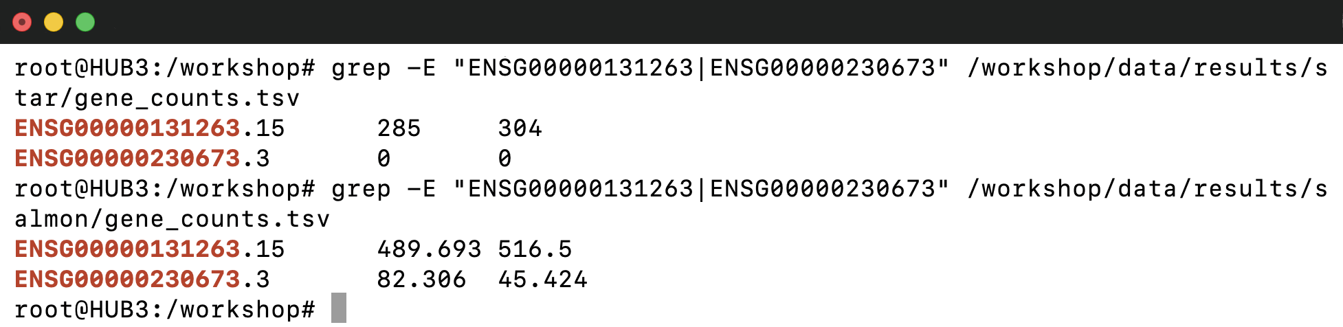

6.3 Interpret agreement and disagreement

Are PABPC1P3’s reads bad? Count all reads over its locus, then just the uniquely mapped ones (MAPQ 255):

samtools view -c        /workshop/data/results/star/ERR188245_Aligned.sortedByCoord.out.bam chrX:74583088-74583546
samtools view -c -q 255 /workshop/data/results/star/ERR188245_Aligned.sortedByCoord.out.bam chrX:74583088-74583546

HUB (Hands-on Understanding of Bioinformatics) Workshop Bulk RNA-seq Data Analysis by Bioinformatics Hub

[Session 3] From FASTQ Files to Gene Counts: Alignment and Quantification.