
HUB (Hands-on
Understanding of Bioinformatics) Workshop
AI-Assisted Bioinformatics
by
Bioinformatics Hub
1 Introduction
1.1 Background
- AI-assisted tools can now support bulk RNA-seq workflows from count matrices through differential expression analysis, thereby increasing the accessibility of these analyses to researchers without extensive bioinformatics training.
- This accessibility also introduces methodological risk. A workflow may produce apparently complete results even when the analyst has limited familiarity with the assumptions underlying individual processing and statistical steps. Consequently, results should be interpreted in relation to the characteristics of the data and the assumptions of the selected methods.
- Zero counts provide a useful example. RNA-seq count matrices commonly contain many zeros, and an observed zero may reflect either negligible biological expression or failure to observe reads at the available sequencing depth. Any transformation must map these zeros onto its transformed scale, and the resulting values can influence subsequent statistical analyses.
- In bulk RNA-seq data, a gene’s standard deviation typically increases with its mean expression: highly expressed genes exhibit greater absolute variability than lowly expressed genes. This mean–variance dependence (heteroscedasticity) can cause highly expressed genes to contribute disproportionately to analyses based on distances or variances when raw counts are used directly.
- Variance-stabilizing normalization (VSN) is designed to reduce this dependence, making variance approximately independent of the mean. It was introduced for microarray intensity data, the dominant expression platform at the time, and implemented in the vsn package, which combines a per-sample affine calibration (a shift and a scale for each sample) with a generalized logarithm (glog2).
- Huber et al. (2002), Bioinformatics. https://doi.org/10.1093/bioinformatics/18.suppl_1.S96
- Huber et al. (2003), Statistical Applications in Genetics and Molecular Biology. https://doi.org/10.2202/1544-6115.1008
- As RNA-seq replaced microarrays as a major expression-profiling platform, the principle of variance stabilization was adapted to count data. The variance-stabilizing transformation (
vst()) of DESeq, and later DESeq2, is derived from the fitted dispersion–mean relationship of a negative binomial model after size-factor normalization, and the DESeq2 documentation cites the vsn work (Huber et al., 2003) among the sources of its variance-stabilizing transformation.- DESeq — Anders and Huber (2010), Genome Biology. https://doi.org/10.1186/gb-2010-11-10-r106
- DESeq2 — Love et al. (2014), Genome Biology. https://doi.org/10.1186/s13059-014-0550-8
- The two methods therefore share one goal but reach it differently:
vsn2()estimates a separate offset and scale for every sample from the data, whereasvst()rescales samples by their size factors and applies one transformation derived from the common dispersion trend. This distinction determines how zero counts are represented on the transformed scale and is the central focus of this report. - The two packages also assume different uses of their output. The DESeq2 documentation states that differential expression is tested on raw counts, and that transformed values are intended for other analyses such as visualization or clustering. The vsn documentation pairs its transformed values with the linear-model tools of limma for differential testing.
1.2 Aims
- To characterize how the variance-stabilizing functions
vst()from the DESeq2 package andvsn2()from the vsn package map zero counts in bulk RNA-seq data onto their transformed scales - To evaluate whether differential expression results obtained from transformed values are associated with differences in the representation of zero counts on the transformed scales
- To compare the differential expression results of the testing route each package documents — DESeq2 applied to the raw counts, and limma applied to the
vsn2()values — and of a Welch t-test applied to the values from both transformations- The Dexamethasone versus Untreated comparison is the primary contrast. Because this treatment effect has been characterized in the published dataset, it provides a common biological setting in which differences among analytical routes can be examined
1.3 Materials
- Gene-level read counts were taken from the airway Bioconductor data package (v1.28.0), which distributes the data from GEO accession GSE52778
- Himes et al. (2014), PLoS One. https://doi.org/10.1371/journal.pone.0099625
- The package authors aligned the paired-end reads with STAR to GRCh37 using Ensembl release 75 annotation and counted fragments per gene with
summarizeOverlaps(union mode, strand ignored) - GSE52778 contains 16 libraries across four treatments (untreated, dexamethasone, albuterol, albuterol plus dexamethasone); the airway package, and therefore this report, contains only the 8 untreated and dexamethasone libraries (4 untreated, 4 dexamethasone)
- A total of 8 samples from four cell lines (N61311, N052611, N080611, N061011), one untreated and one dexamethasone-treated library per cell line (Untreated: 4; Dexamethasone: 4):
- Untreated — ◼ untreated airway smooth muscle cells (control)
- Dexamethasone — ◼ cells treated with the glucocorticoid dexamethasone
1.4 Computational Methods
- The workflow comprised data retrieval, filtering, two variance-stabilizing transformations, four differential expression tests and a comparison of their results:
- The count matrix was retrieved from the airway data package (v1.28.0) and loaded in R
- Size-factor normalization, the variance-stabilizing transformation, and the reference differential expression test on raw counts used DESeq2 (v1.48.2)
- Per-sample calibration and glog2 transformation used vsn (v3.76.0)
- Moderated linear-model testing of the
vsn2()values used limma (v3.64.3) - Two-sample testing of the transformed values used the Welch t-test, as implemented in base R
- p-values from every test were adjusted with the Benjamini–Hochberg procedure
2 Data Characteristics
2.1 Raw Count Distributions
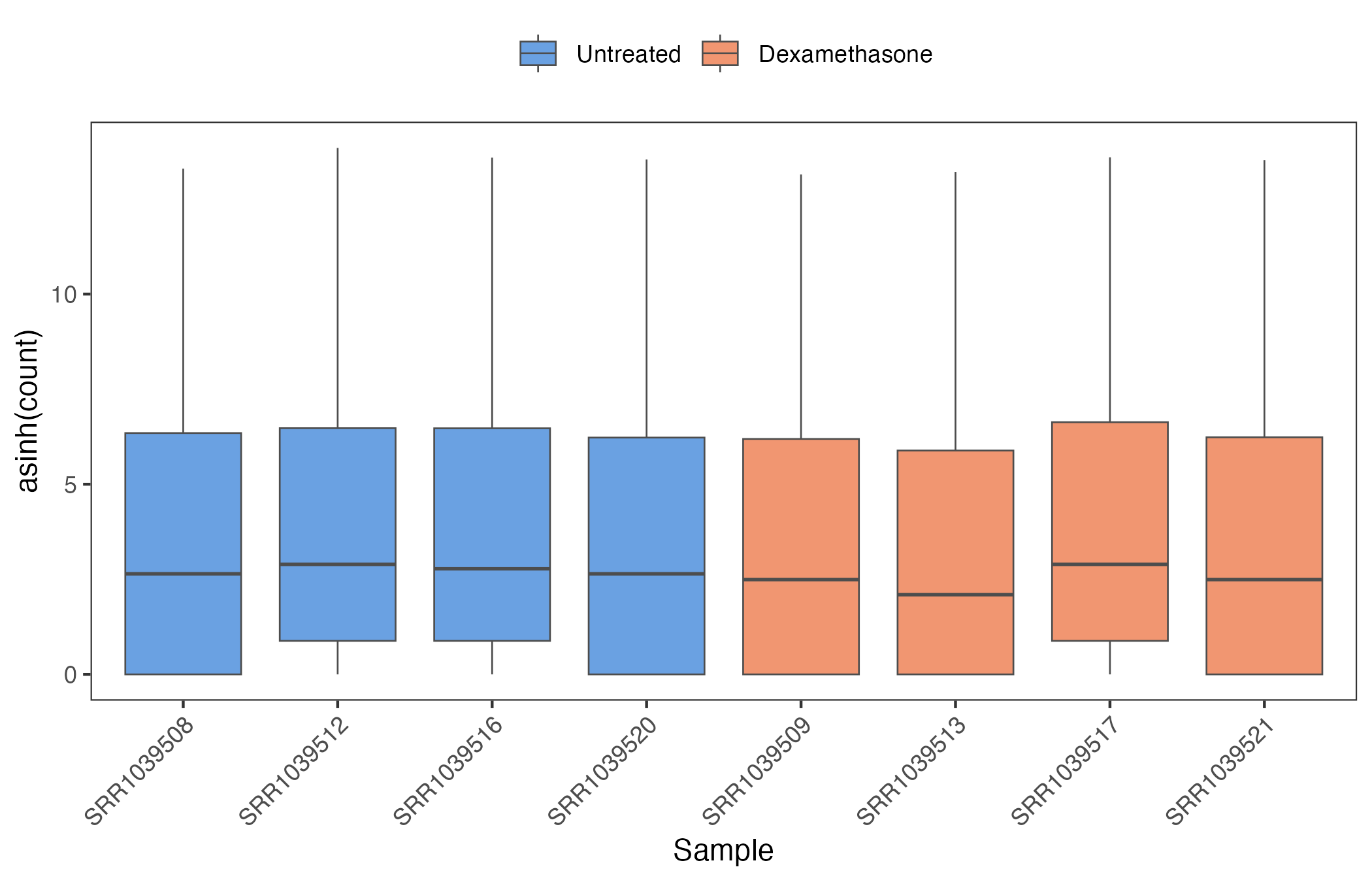
- Summary: The 8 libraries contain between 15.16 and 30.82 million assigned fragments. After genes with zero counts in every sample were removed, each library still contained between 7,471 and 10,345 zero counts (22.3–30.9% of the 33,469 retained genes).
- The panels show the 33,469 of 63,677 genes retained after filtering (30,208 genes with zero counts in all 8 samples removed); the filtering step itself is described under Transformation and Testing
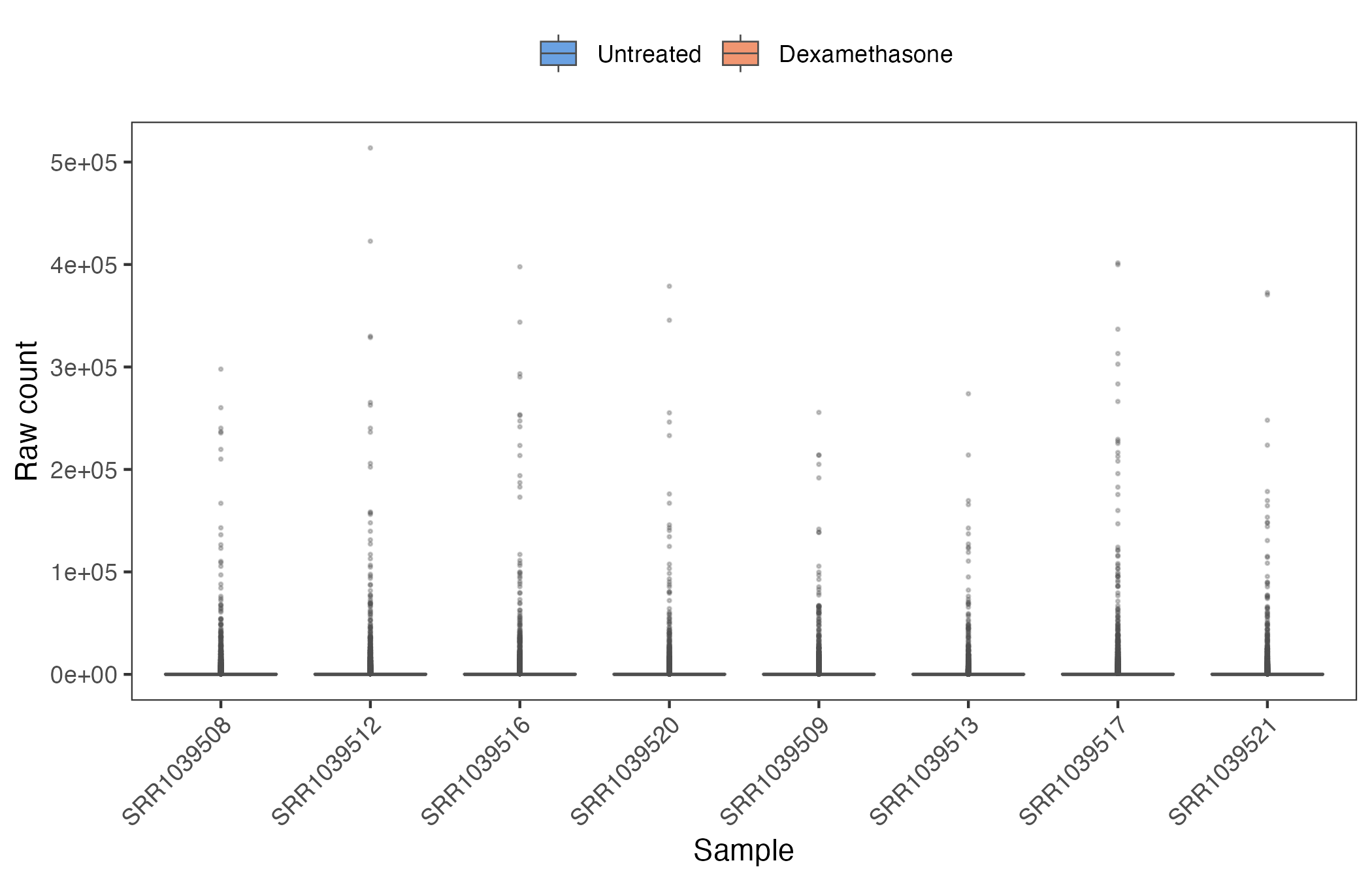
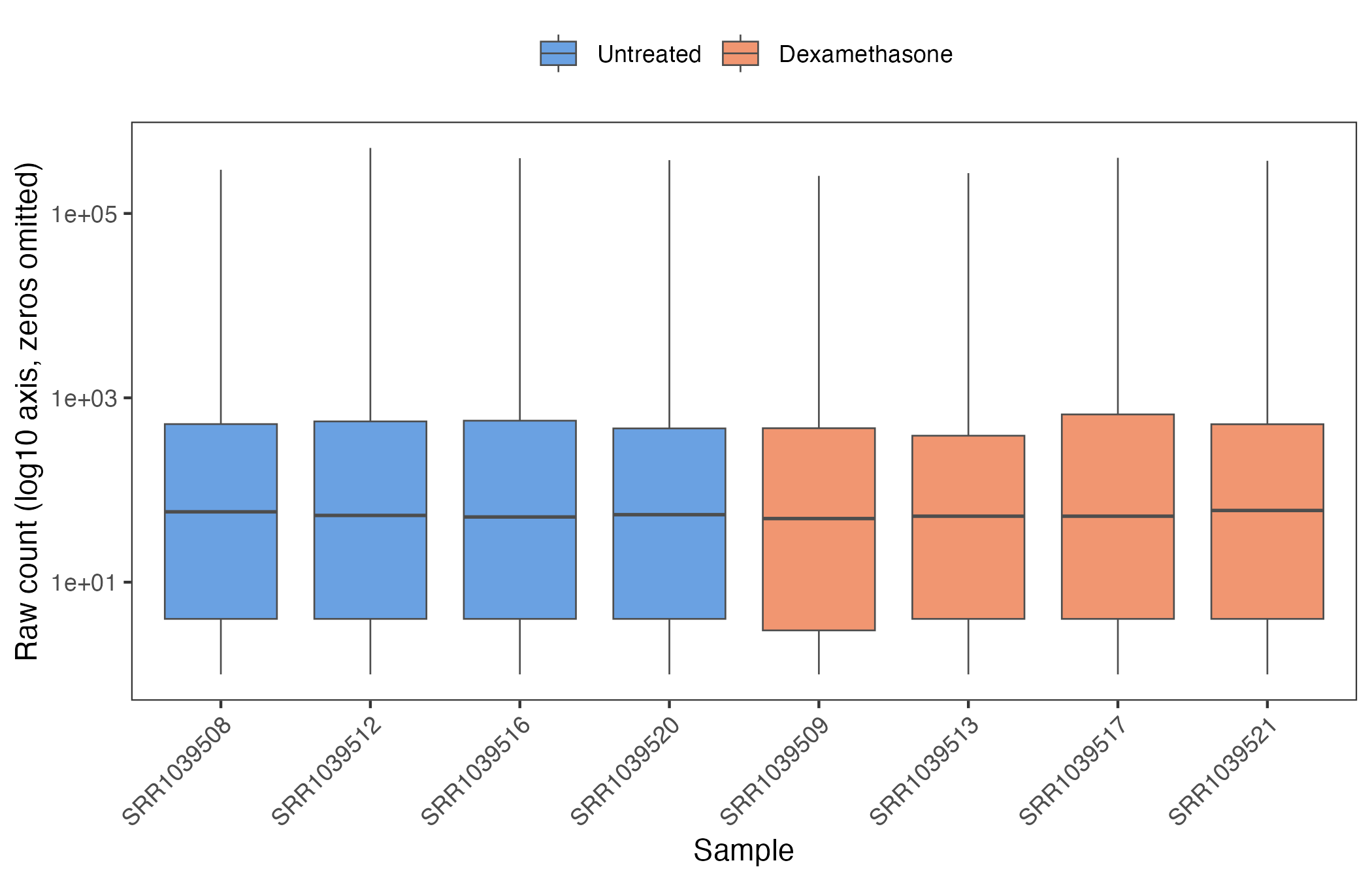
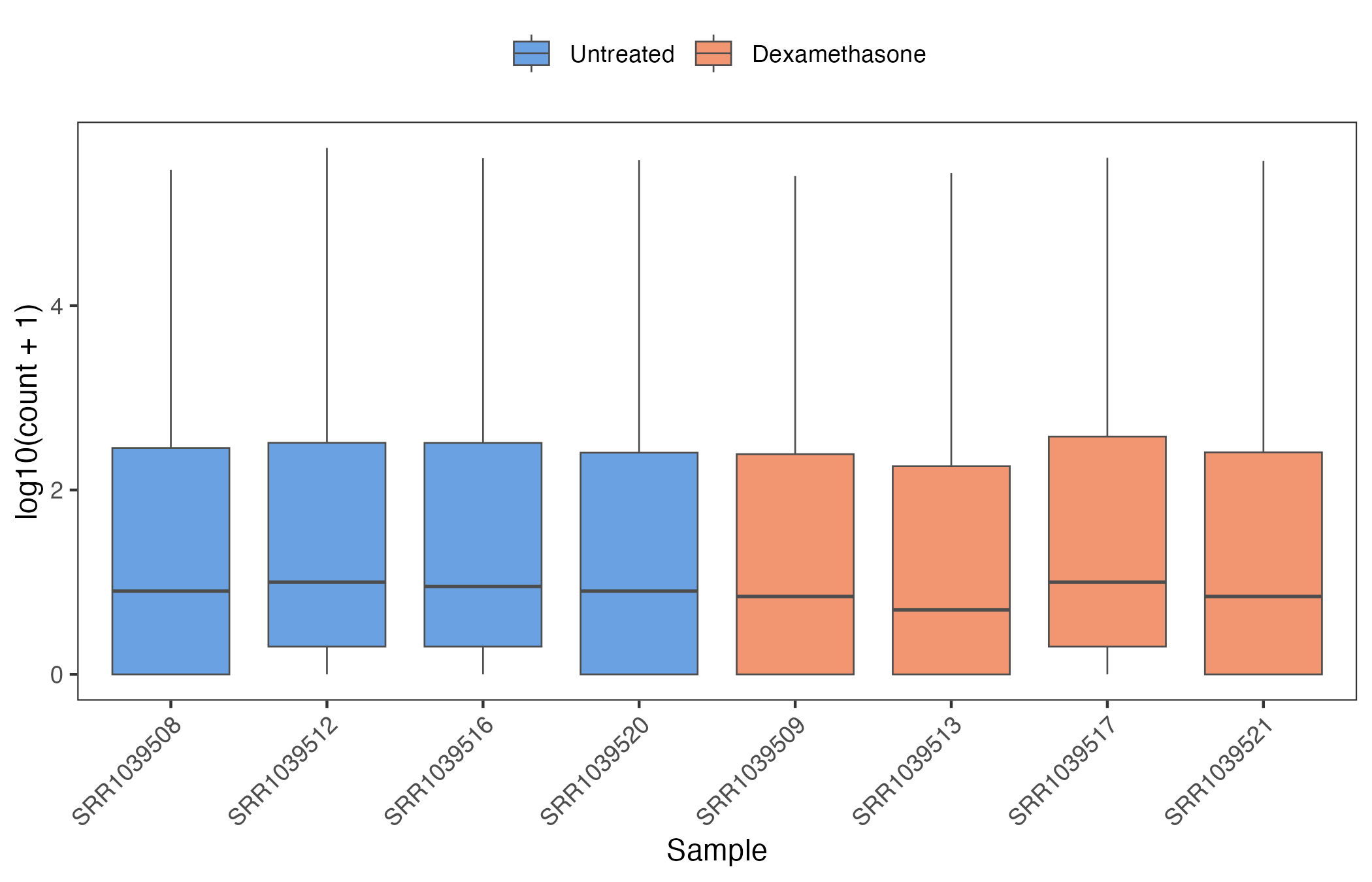
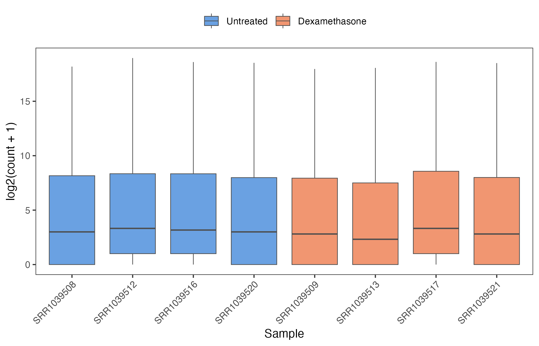
- The same raw counts are displayed on five scales to illustrate how the representation of zero values depends on the chosen scale
- Interpretation:
- Raw count — raw counts on a linear axis; a small number of highly expressed genes determine the plotting range, compressing the boxplots near zero
- log10 axis — the axis is logarithmic but the values are unchanged; zeros cannot be drawn on a log axis and are left out (69,610 of 267,752 values)
- log10(count + 1) — a pseudocount of 1 keeps zeros at 0 on a base-10 scale; the lower quartile is 0 in the same five samples
- log2(count + 1) — a pseudocount of 1 keeps zeros at 0; the lower quartile is 0 in five of the eight samples
- asinh(count) — the inverse hyperbolic sine, which is 0 at 0 and close to a logarithm for large counts; it is the functional form underlying the vsn glog
2.1.1 Raw count
2.1.2 log10 axis
2.1.3 log10(count + 1)
2.1.4 log2(count + 1)
2.1.5 asinh(count)
2.2 Mean–Variance Relationship
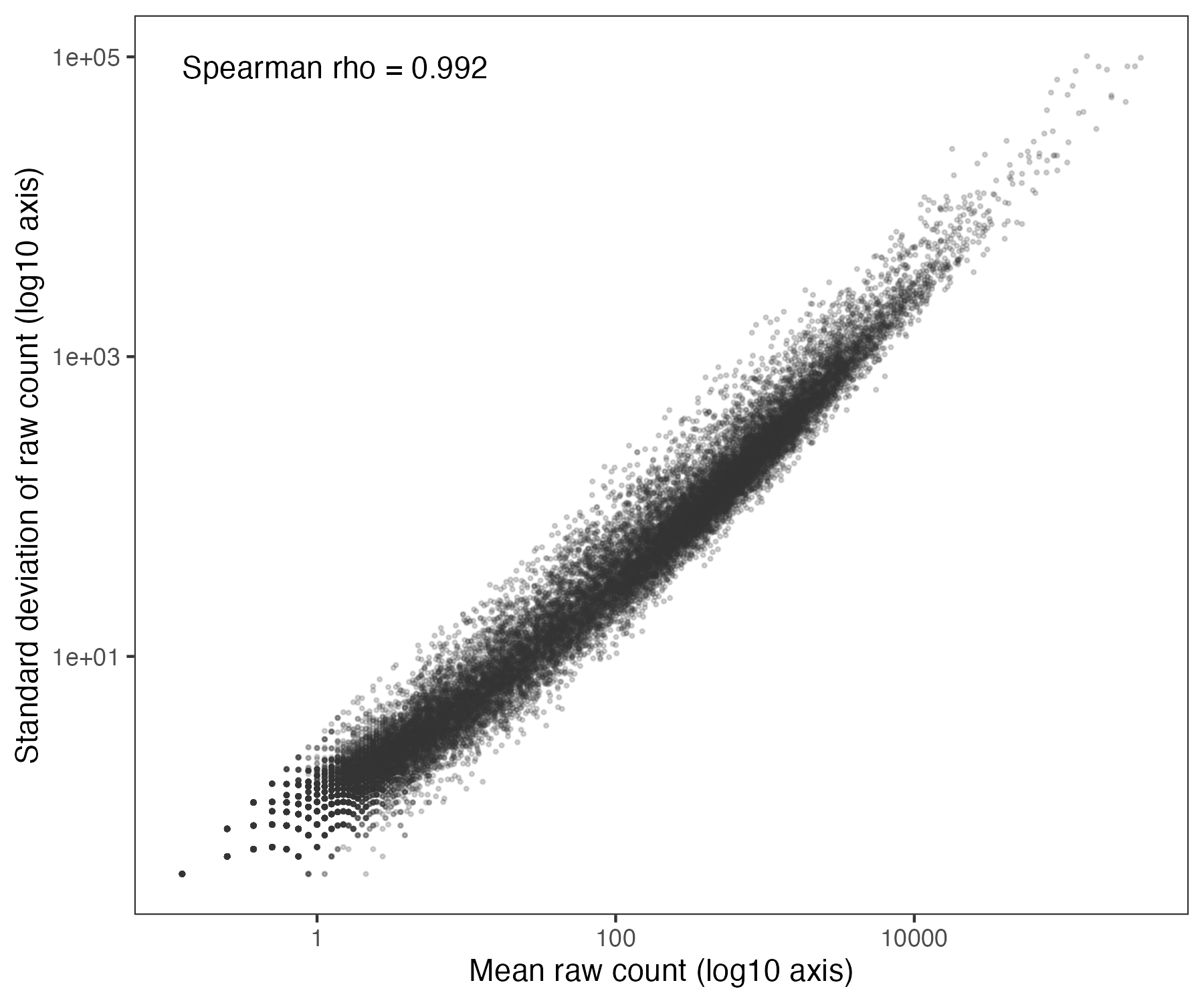
- Summary: Across the 33,469 retained genes, the standard deviation of the raw counts increases with the mean over mean counts ranging from 0.125 to approximately 329,000 (Spearman rho = 0.992). This strong association illustrates the mean–variance dependence described above: on the raw-count scale, highly expressed genes exhibit greater absolute variability, motivating the use of variance-stabilizing transformations for analyses based on distances or variances.
- Each dot is one gene: its mean raw count across the 8 libraries (x-axis) against the standard deviation of those counts (y-axis)
- Both axes are on a log10 scale, because gene means range from 0.125 to about 329,000 counts; no gene has a standard deviation of 0, so every gene is shown
- Raw counts were used, without size-factor normalization, so the panel shows the data exactly as they enter the transformations
- Interpretation:
- Rising diagonal band — the spread of a gene grows with its expression level; a variance-stabilized scale would instead show a roughly flat band
- Discrete grid at the lower left — genes with only a few reads can take only a few distinct combinations of counts (0, 1, 2 …), so their mean and standard deviation fall on a lattice; these are the genes in which zeros are concentrated
- Spearman rho — rank correlation between mean and standard deviation across genes; 1 means the two always increase together
2.3 Zero-Count Distribution
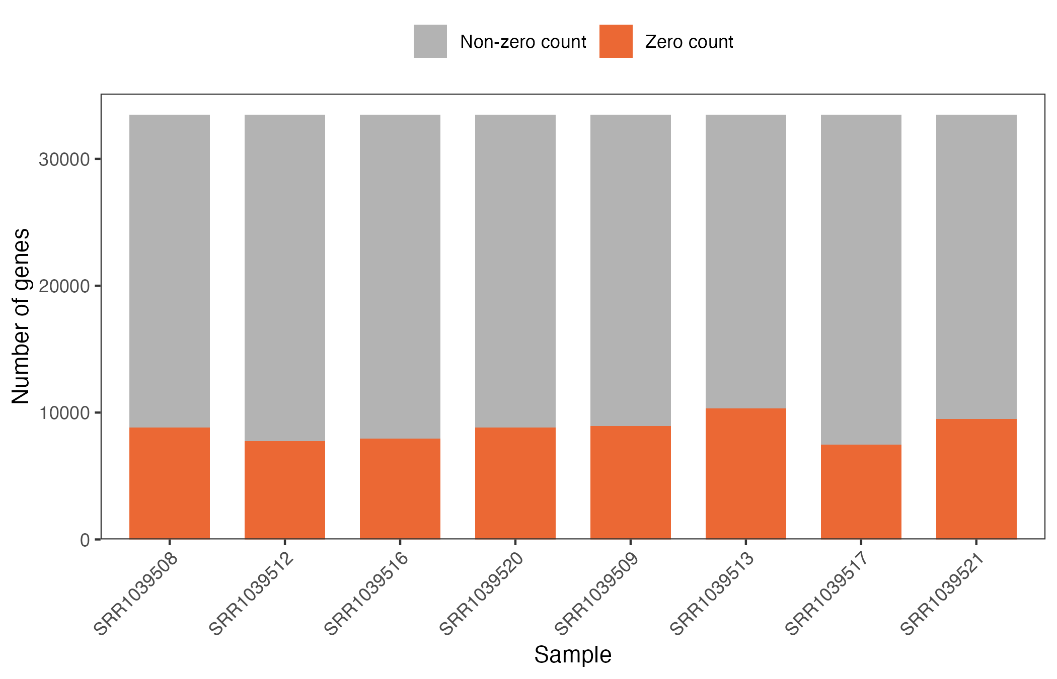
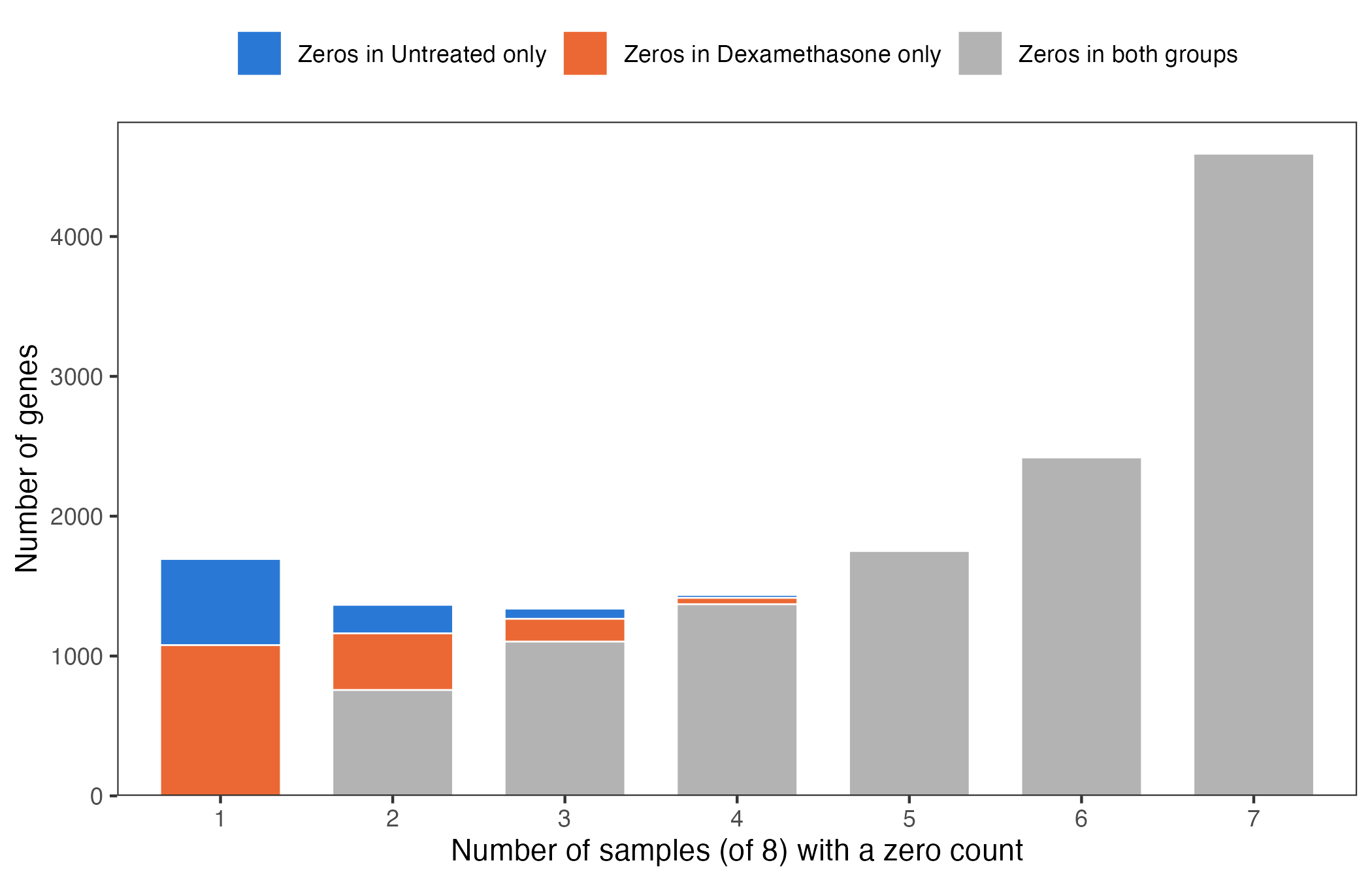
- Summary: Per sample, between 7,471 (SRR1039517) and 10,345 (SRR1039513) of the 33,469 retained genes have a zero count; the Untreated libraries range from 7,770 to 8,836 and the Dexamethasone libraries from 7,471 to 10,345. Of the 33,469 retained genes, 14,599 (43.6%) have a zero count in at least one sample, and the most common pattern is a gene with reads in only one sample (zero in 7 of 8; 4,592 genes). In 2,606 genes the zeros fall in one treatment group only, and these are unevenly split: 1,692 have zeros in Dexamethasone only against 914 in Untreated only. Sixty-seven genes are zero in all four libraries of one group and non-zero in all four of the other (46 in Dexamethasone, 21 in Untreated).
- Per sample — one bar per library, Untreated libraries left and Dexamethasone libraries right, split into genes with a zero count (orange) and genes with a non-zero count (grey); every bar totals the 33,469 retained genes
- Per gene — each bar counts the genes that have a zero count in a given number of the 8 samples, split by where the zeros fall (Untreated only, Dexamethasone only, or both groups); the 18,870 genes with no zero (56.4% of the 33,469 retained genes) are not shown
- Interpretation:
- Zeros in both groups — predominantly low-count genes with intermittent detection across both treatment groups; this pattern does not, by itself, indicate a systematic between-group difference
- Zeros in one group only — a pattern that can contribute to an apparent between-group difference in a two-group analysis; the greater frequency of Dexamethasone-only zeros is consistent with the higher zero burden observed in several Dexamethasone libraries, particularly SRR1039513
- Seven of eight samples zero — genes with reads detected in only one library; although retained by the zero-in-all-samples filter, these genes contain very limited information for estimating a treatment effect
2.3.1 Per sample
2.3.2 Per gene
3 Transformation and Testing
3.1 Environment Settings
- Summary: The treatment groups, their colours, the significance threshold and the R packages used by every analysis below are set here, so the code in this section runs on its own in an R session.
group_orderfixes the order of the two treatment groups in tables and figures, andgroup_colstheir coloursFDRis the adjusted p-value threshold applied to all four routes, andsig()marks a gene as significant when its adjusted p-value is below it- The packages provide the airway data (airway, SummarizedExperiment), the transformations and tests (DESeq2, vsn, limma) and the figures (ggplot2, ggVennDiagram)
suppressPackageStartupMessages({
        library(airway)
        library(SummarizedExperiment)
        library(DESeq2)
        library(vsn)
        library(limma)
        library(ggplot2)
        library(ggVennDiagram)
})

# Treatment groups, in plotting order, and their colours
group_order <- c("Untreated", "Dexamethasone")
group_cols  <- c(Untreated = "#2a78d6", Dexamethasone = "#eb6834")

# Significance threshold (adjusted p-value), applied identically to all four routes
FDR <- 0.05

# A gene is significant when its adjusted p-value is below FDR; NA counts as not significant
sig <- function(p) !is.na(p) & p < FDR
3.2 Count Matrix Overview
- Summary: The gene-level count matrix and the sample annotation are loaded from the airway package; together they are the single input to every analysis below.
countsholds one row per Ensembl gene and one column per librarysamplesrecords the cell line and treatment group of each library
data(airway, package = "airway")
counts <- assay(airway, "counts")
samples <- data.frame(
        sample = colnames(airway),
        cell = as.character(airway$cell),
        group = ifelse(as.character(airway$dex) == "trt", "Dexamethasone", "Untreated")
)
group <- factor(samples$group, levels = group_order)
names(group) <- samples$sample

dim(counts)
## [1] 63677 8head(counts)## SRR1039508 SRR1039509 SRR1039512 SRR1039513 SRR1039516
## ENSG00000000003 679 448 873 408 1138
## ENSG00000000005 0 0 0 0 0
## ENSG00000000419 467 515 621 365 587
## ENSG00000000457 260 211 263 164 245
## ENSG00000000460 60 55 40 35 78
## ENSG00000000938 0 0 2 0 1
## SRR1039517 SRR1039520 SRR1039521
## ENSG00000000003 1047 770 572
## ENSG00000000005 0 0 0
## ENSG00000000419 799 417 508
## ENSG00000000457 331 233 229
## ENSG00000000460 63 76 60
## ENSG00000000938 0 0 0dim(samples)## [1] 8 3head(samples)| sample | cell | group |
|---|---|---|
| SRR1039508 | N61311 | Untreated |
| SRR1039509 | N61311 | Dexamethasone |
| SRR1039512 | N052611 | Untreated |
| SRR1039513 | N052611 | Dexamethasone |
| SRR1039516 | N080611 | Untreated |
| SRR1039517 | N080611 | Dexamethasone |
3.3 Gene Filtering
- Summary: Of the 63,677 genes, 30,208 (47.4%) had zero counts in all 8 samples and were removed, leaving 33,469 genes for every later step.
- Genes with zero counts in every sample provide no between-sample information for the transformations or tests considered here and were therefore removed
- No additional expression filter was applied, thereby retaining low-count genes for which the treatment of zero values is most consequential
keep <- rowSums(counts) > 0
filtered <- counts[keep, ]

dim(filtered)
## [1] 33469 83.4 Zero-Value Statistics
- Summary: After filtering, 69,610 of 267,752 values (26.0%) are zero. A total of 14,599 genes contain at least one zero, including 2,606 genes in which zeros occur exclusively in one treatment group. Such one-sided zero patterns can contribute to between-group differences in analyses of transformed values.
- The first table gives the number and fraction of zeros in each library
- The second table classifies each gene by where its zeros occur
zero_samples <- data.frame(
        Sample = colnames(filtered),
        Group = group[colnames(filtered)],
        `Library size` = colSums(filtered),
        Zeros = colSums(filtered == 0),
        `Zero fraction (%)` = round(100 * colMeans(filtered == 0), 1),
        check.names = FALSE
)
zero_samples| Sample | Group | Library size | Zeros | Zero fraction (%) |
|---|---|---|---|---|
| SRR1039508 | Untreated | 20,637,971 | 8,836 | 26.4 |
| SRR1039509 | Dexamethasone | 18,809,481 | 8,942 | 26.7 |
| SRR1039512 | Untreated | 25,348,649 | 7,770 | 23.2 |
| SRR1039513 | Dexamethasone | 15,163,415 | 10,345 | 30.9 |
| SRR1039516 | Untreated | 24,448,408 | 7,961 | 23.8 |
| SRR1039517 | Dexamethasone | 30,818,215 | 7,471 | 22.3 |
| SRR1039520 | Untreated | 19,126,151 | 8,807 | 26.3 |
| SRR1039521 | Dexamethasone | 21,164,133 | 9,478 | 28.3 |
zeros_untrt <- rowSums(filtered[, group == group_order[1]] == 0)
zeros_dex <- rowSums(filtered[, group == group_order[2]] == 0)
zero_pattern <- ifelse(zeros_untrt + zeros_dex == 0, "No zeros",
                ifelse(zeros_untrt > 0 & zeros_dex > 0, "Zeros in both groups",
                ifelse(zeros_untrt > 0, "Zeros in Untreated only", "Zeros in Dexamethasone only")))
zero_pattern <- factor(zero_pattern, levels = c("No zeros", "Zeros in both groups",
                                                "Zeros in Untreated only", "Zeros in Dexamethasone only"))
zero_pattern_counts <- data.frame(`Zero pattern` = levels(zero_pattern), Genes = as.vector(table(zero_pattern)),
                                  check.names = FALSE)
zero_pattern_counts| Zero pattern | Genes |
|---|---|
| No zeros | 18,870 |
| Zeros in both groups | 11,993 |
| Zeros in Untreated only | 914 |
| Zeros in Dexamethasone only | 1,692 |
3.5 Variance-Stabilizing Transformations
- Summary: Both transformations were applied to the same 33,469 filtered genes; the subsections below compare where each placed the 69,610 zero counts.
- DESeq2 first estimates a size factor for each library (median-of-ratios normalization), then fits the relationship between each gene’s mean and its dispersion, and derives from that fit a transformation whose output has approximately constant variance and is on a log2-like scale for large counts
blind = TRUEignores the group labels when estimating dispersions; this is the DESeq2 default and its recommendation for quality assessment- The design
~ groupis recorded in the object only because the same object is later used for testing; it does not affect the blind transformation
- vsn fits, for each sample, an affine calibration (an offset and a scaling factor) and then applies a glog2 transformation, estimating all parameters jointly by robust maximum likelihood under the assumption that most genes are not differentially expressed
vsn2()was run with its default settings on the filtered raw counts; the calibrated and transformed values are read from thehxslot
dds <- DESeqDataSetFromMatrix(filtered, data.frame(group = group, row.names = names(group)), ~group)
vst_obj <- vst(dds, blind = TRUE)
vst_mat <- assay(vst_obj)

head(vst_mat)
## SRR1039508 SRR1039509 SRR1039512 SRR1039513 SRR1039516
## ENSG00000000003 9.463462 9.083112 9.612635 9.347635 9.978952
## ENSG00000000419 8.961712 9.269663 9.152274 9.197839 9.079201
## ENSG00000000457 8.208122 8.114127 8.047259 8.162081 7.962763
## ENSG00000000460 6.601433 6.643869 6.141319 6.497653 6.715452
## ENSG00000000938 4.436956 4.436956 4.839310 4.436956 4.722142
## ENSG00000000971 11.652429 12.018364 12.366393 12.641376 12.489412
## SRR1039517 SRR1039520 SRR1039521
## ENSG00000000003 9.627714 9.779777 9.340292
## ENSG00000000419 9.261302 8.952013 9.180790
## ENSG00000000457 8.120108 8.203470 8.150363
## ENSG00000000460 6.369401 6.930898 6.676050
## ENSG00000000938 4.436956 4.436956 4.436956
## ENSG00000000971 12.952216 12.467750 13.054593vsn_fit <- vsn2(filtered)
vsn_mat <- vsn_fit@hx
head(vsn_mat)## SRR1039508 SRR1039509 SRR1039512 SRR1039513 SRR1039516
## ENSG00000000003 9.3877132 8.9815582 9.522508 9.2727246 9.917072
## ENSG00000000419 8.8492157 9.1820610 9.032284 9.1124923 8.964068
## ENSG00000000457 8.0081012 7.9002227 7.798232 7.9634031 7.709425
## ENSG00000000460 5.9208581 5.9865813 5.133182 5.7688873 6.079794
## ENSG00000000938 0.6111713 0.6216318 1.653383 0.6817389 1.216593
## ENSG00000000971 11.6445102 12.0154425 12.342893 12.6508412 12.477417
## SRR1039517 SRR1039520 SRR1039521
## ENSG00000000003 9.5746013 9.6889425 9.2702746
## ENSG00000000419 9.1854709 8.8063566 9.0995492
## ENSG00000000457 7.9192514 7.9704640 7.9550810
## ENSG00000000460 5.5626693 6.3719791 6.0482064
## ENSG00000000938 0.5581231 0.5909049 0.6492472
## ENSG00000000971 12.9687869 12.4356088 13.07188193.5.1 vst transformation
- Summary: Under
vst(), every zero count was mapped to the same transformed value, 4.437, in all 8 samples. This occurs because size-factor normalization leaves a zero unchanged, whereas non-zero counts are rescaled according to sample-specific size factors, which ranged from 0.67 to 1.40. - The table gives each library’s size factor and the single value its zero counts were transformed to
vst_zero_values <- data.frame(
        Sample = colnames(filtered),
        `Size factor` = round(vst_obj$sizeFactor, 3),
        `Value of 0` = sapply(colnames(filtered), function(j) round(unique(vst_mat[filtered[, j] == 0, j]), 3)),
        check.names = FALSE
)
vst_zero_values| Sample | Size factor | Value of 0 |
|---|---|---|
| SRR1039508 | 1.024 | 4.437 |
| SRR1039509 | 0.896 | 4.437 |
| SRR1039512 | 1.179 | 4.437 |
| SRR1039513 | 0.670 | 4.437 |
| SRR1039516 | 1.178 | 4.437 |
| SRR1039517 | 1.399 | 4.437 |
| SRR1039520 | 0.921 | 4.437 |
| SRR1039521 | 0.945 | 4.437 |
3.5.2 vsn transformation
- Summary: Under
vsn2(), zero counts were mapped to values ranging from 0.551 to 0.682. All zeros within a given sample received the same value, whereas the value differed among samples becausevsn2()estimates a sample-specific offset and scale before transformation. - The table gives each library’s fitted calibration offset and scale and the value its zero counts were transformed to
vsn_zero_values <- data.frame(
        Sample = colnames(filtered),
        Offset = round(coef(vsn_fit)[1, , 1], 3),
        Scale = round(coef(vsn_fit)[1, , 2], 3),
        `Value of 0` = sapply(colnames(filtered), function(j) round(unique(round(vsn_mat[filtered[, j] == 0, j], 6)), 3)),
        check.names = FALSE
)
vsn_zero_values| Sample | Offset | Scale | Value of 0 |
|---|---|---|---|
| SRR1039508 | 18.005 | 2.452 | 0.611 |
| SRR1039509 | 18.137 | 2.586 | 0.622 |
| SRR1039512 | 17.265 | 2.294 | 0.551 |
| SRR1039513 | 18.909 | 2.881 | 0.682 |
| SRR1039516 | 17.399 | 2.303 | 0.562 |
| SRR1039517 | 17.354 | 2.149 | 0.558 |
| SRR1039520 | 17.754 | 2.535 | 0.591 |
| SRR1039521 | 18.488 | 2.542 | 0.649 |
3.5.3 Per-sample boxplots
- Summary: On the shared axis, the lower whisker of each
vst()distribution occurs at 4.437, whereas the correspondingvsn2()values range from 0.551 to 0.682. These positions reflect the transformed values assigned to zero counts; numerically, thevst()zero value is approximately 3.8 units higher on the displayed scale. - One box per library, coloured by treatment group, for the
vst()values (first tab), thevsn2()values (second tab) and the raw counts on a log2(count + 1) scale (third tab) - Libraries are ordered as in 2.1, Untreated on the left and Dexamethasone on the right
- All three panels use the same y-axis limits so that the scales can be compared directly; on the log2(count + 1) scale a zero stays at 0
to_long <- function(m) {
        data.frame(
                sample = factor(rep(colnames(m), each = nrow(m)), levels = sample_order),
                group = rep(group[colnames(m)], each = nrow(m)),
                value = as.vector(m)
        )
}
sample_order <- names(group)[order(group)]
raw_log2 <- log2(filtered + 1)
value_limits <- range(c(vst_mat, vsn_mat, raw_log2))

# per-gene mean and standard deviation on each scale, used in the mean-variance panel
mean_sd <- rbind(
        data.frame(scale = "Raw", mean = log2(rowMeans(filtered) + 1), sd = log2(apply(filtered, 1, sd) + 1)),
        data.frame(scale = "vsn", mean = rowMeans(vsn_mat), sd = apply(vsn_mat, 1, sd)),
        data.frame(scale = "vst", mean = rowMeans(vst_mat), sd = apply(vst_mat, 1, sd))
)
# drawing order: raw first, vsn last (on top)
mean_sd$scale <- factor(mean_sd$scale, levels = c("Raw", "vst", "vsn"))
scale_cols <- c(Raw = "grey20", vst = "#c51b8a", vsn = "#0b8fb3")
msd_rho <- sapply(split(mean_sd, mean_sd$scale), function(d) cor(d$mean, d$sd, method = "spearman"))
msd_sd_range <- lapply(split(mean_sd$sd, mean_sd$scale), range)
theme_report <- theme_bw(base_size = 11) +
        theme(panel.grid.major = element_blank(), panel.grid.minor = element_blank(),
              legend.position = "top")

box_plot <- function(m, ylab) {
        ggplot(to_long(m), aes(x = sample, y = value, fill = group)) +
                geom_boxplot(colour = "grey30", linewidth = 0.3, alpha = 0.7,
                             outlier.size = 0.3, outlier.alpha = 0.3) +
                scale_fill_manual(values = group_cols, name = NULL) +
                scale_y_continuous(limits = value_limits) +
                labs(x = "Sample", y = ylab) +
                theme_report +
                theme(axis.text.x = element_text(angle = 45, hjust = 1))
}

dens_plot <- function(m, xlab) {
        ggplot(to_long(m), aes(x = value, group = sample, colour = group)) +
                geom_density(linewidth = 0.5) +
                scale_colour_manual(values = group_cols, name = NULL) +
                scale_x_continuous(limits = value_limits) +
                labs(x = xlab, y = "Density") +
                theme_report
}
3.5.3.1 vst
box_plot(vst_mat, "vst (log2 scale)")
3.5.3.2 vsn
box_plot(vsn_mat, "vsn (glog2 scale)")
3.5.3.3 Raw count
box_plot(raw_log2, "log2(count + 1)")
3.5.4 Density
- Summary: Under both transformations, zero counts form a distinct peak at the lower end of each density distribution, centered near 4.4 for
vst()and 0.6 forvsn2(), compared with 0 on the log2(count + 1) scale. Non-zero counts form a broader distribution at higher transformed values. - One density curve per library, coloured by treatment group, for the
vst()values (first tab), thevsn2()values (second tab) and the raw counts on a log2(count + 1) scale (third tab) - All three panels use the same x-axis limits
3.5.4.1 vst
dens_plot(vst_mat, "vst (log2 scale)")
3.5.4.2 vsn
dens_plot(vsn_mat, "vsn (glog2 scale)")
3.5.4.3 Raw count
dens_plot(raw_log2, "log2(count + 1)")
3.5.5 Mean–variance relationship
- Summary: For the raw counts, the log2-scaled standard deviation increases strongly with the log2-scaled mean (Spearman rho = 0.992), ranging from 0.44 to 16.62. Following transformation, the standard deviation is restricted to 0.025–3.43 for
vst()and 0.027–5.06 forvsn2(), with substantially weaker mean–variance associations (Spearman rho = 0.354 and -0.223, respectively). - Each dot is one gene: its mean across the 8 libraries (x-axis) against the standard deviation across the same libraries (y-axis), on the
vst()scale (magenta), thevsn2()scale (cyan) and for the raw counts (grey, as in 2.2) - For the raw counts, the mean and standard deviation are each shown as log2(value + 1), so that all three scales fit on the same linear axes;
vst()andvsn2()values are shown as they are - The raw counts are drawn first, then
vst(), thenvsn2(), so where they overlapvsn2()is on top - Interpretation:
- Approximately flat band — the expected pattern after successful variance stabilization, in which the standard deviation shows substantially reduced dependence on the mean
- Rising grey band — on the raw scale, more highly expressed genes vary more in absolute counts, as in 2.2
- Spearman rho — rank correlation between mean and standard deviation across genes for each scale; values near 0 mean the spread no longer tracks the expression level
ggplot(mean_sd, aes(x = mean, y = sd, colour = scale)) +
        geom_point(size = 0.3, alpha = 0.15) +
        scale_colour_manual(values = scale_cols, labels = c("Raw count", "vst", "vsn"), name = NULL) +
        guides(colour = guide_legend(override.aes = list(size = 3, alpha = 1))) +
        labs(x = "Mean across libraries", y = "Standard deviation across libraries") +
        theme_report
3.6 Statistical Testing
dds <- DESeq(dds, quiet = TRUE)
res <- results(dds, alpha = FDR)
filter_threshold <- metadata(res)$filterThreshold

welch_p <- function(m) {
        apply(m, 1, function(r) {
                a <- r[group == group_order[1]]
                b <- r[group == group_order[2]]
                if (var(a) == 0 && var(b) == 0) return(NA_real_)
                t.test(a, b)$p.value
        })
}
padj_vst_welch <- p.adjust(welch_p(vst_mat), "BH")
padj_vsn_welch <- p.adjust(welch_p(vsn_mat), "BH")

design <- model.matrix(~group)
fit <- eBayes(lmFit(vsn_mat, design))
lim <- topTable(fit, coef = 2, number = Inf, sort.by = "none")
padj_vsn_limma <- lim$adj.P.Val

head(as.data.frame(res))| baseMean | log2FoldChange | lfcSE | stat | pvalue | padj | |
|---|---|---|---|---|---|---|
| ENSG00000000003 | 708.6021697 | -0.3788467 | 0.1731411 | -2.1880804 | 0.0286637 | 0.1387715 |
| ENSG00000000419 | 520.2979006 | 0.2037605 | 0.1005987 | 2.0254789 | 0.0428182 | 0.1826292 |
| ENSG00000000457 | 237.1630368 | 0.0340429 | 0.1262790 | 0.2695852 | 0.7874794 | 0.9301523 |
| ENSG00000000460 | 57.9326331 | -0.1171781 | 0.3012365 | -0.3889904 | 0.6972833 | 0.8945814 |
| ENSG00000000938 | 0.3180984 | -1.7245689 | 3.4936334 | -0.4936319 | 0.6215662 | NA |
| ENSG00000000971 | 5,817.3528677 | 0.4409598 | 0.2589239 | 1.7030477 | 0.0885591 | 0.2981093 |
head(lim)| logFC | AveExpr | t | P.Value | adj.P.Val | B | |
|---|---|---|---|---|---|---|
| ENSG00000000003 | -0.3542690 | 9.4519242 | -2.0174093 | 0.0772206 | 0.4195431 | -4.783590 |
| ENSG00000000419 | 0.2319123 | 9.0289372 | 2.0276322 | 0.0759918 | 0.4160592 | -4.768504 |
| ENSG00000000457 | 0.0629340 | 7.9030226 | 0.5216676 | 0.6155841 | 0.8278613 | -6.449809 |
| ENSG00000000460 | -0.0348674 | 5.8590198 | -0.1313079 | 0.8986707 | 0.9590769 | -6.587618 |
| ENSG00000000938 | -0.3903278 | 0.8228492 | -1.6056575 | 0.1457905 | 0.5564550 | -5.365638 |
| ENSG00000000971 | 0.4516308 | 12.4509227 | 1.6008029 | 0.1468625 | 0.5584779 | -5.372135 |
3.6.1 DESeq2 on raw counts
Summary: DESeq2 called 2,700 genes differentially expressed at adjusted p < 0.05. Its independent filtering gave 14,924 genes with a mean normalized count below 3.743 a nominal p-value but no adjusted p-value, and its count-outlier detection (Cook’s distance) gave a further 51 genes neither; 14,975 genes in all have an adjusted p of NA.
The DESeq2 authors state that differential expression is tested on the raw counts, and that transformed values such as
vst()are for other downstream uses, e.g. visualization or clustering (quality control), not for testing:In order to test for differential expression, we operate on raw counts and use discrete distributions … However for other downstream analyses – e.g. for visualization or clustering – it might be useful to work with transformed versions of the count data.
The table breaks the 33,469 genes into significant, tested but not significant, and adjusted p-value = NA
- Independent filtering (default in
results()): genes with a low mean normalized count have a nominal p-value but an adjusted p-value of NA, because DESeq2 leaves them out of the Benjamini–Hochberg adjustment - The authors’ rationale is that low-count genes have little power to reach significance, so removing them reduces the multiple-testing burden on the rest; because the filter ignores the group labels, they treat it as independent of the test statistic under the null hypothesis Bourgon et al. (2010)
- Independent filtering (default in
deseq2_outcome <- data.frame(
        `DESeq2 outcome` = c("Significant", "Tested, not significant", "Adjusted *p*-value = NA"),
        Genes = c(sum(sig(res$padj)), sum(!is.na(res$padj) & !sig(res$padj)), sum(is.na(res$padj))),
        check.names = FALSE
)
deseq2_outcome| DESeq2 outcome | Genes |
|---|---|
| Significant | 2,700 |
| Tested, not significant | 15,794 |
| Adjusted p-value = NA | 14,975 |
3.6.2 Welch t-test and limma
- Summary: The Welch t-test called 223 genes significant on
vst()values and 203 onvsn2()values. On thevsn2()values, limma called 864. - Two comparisons are made, one per tab:
- Same test, different data profiles (first tab):
vst()andvsn2()differ in their treatment of zeros and mean–variance dependence. Applying the same Welch t-test to both profiles isolates differences associated with the transformed data representation while holding the test procedure constant. The 2,700 genes called by DESeq2 on the raw counts (3.6.1) are shown alongside - Same data profile, different tests (second tab): the same
vsn2()values are analyzed using the Welch t-test and limma. This comparison holds the transformed data profile constant and therefore highlights differences associated with the statistical testing procedure.
- Same test, different data profiles (first tab):
- The two data profiles:
vst()values — size-factor scaling followed by a transformation derived from the fitted dispersion–mean relationship; every zero is mapped to the same valuevsn2()values — a per-sample offset and scale followed by a glog2 transformation; zeros are mapped to a different value in each sample
- The two tests:
- Welch t-test — compares the two group means gene by gene, without assuming equal variances and without sharing information across genes, so each gene’s variance is estimated from its own 8 values Welch (1947)
- limma — fits a linear model per gene and shrinks each gene’s variance towards a common value (empirical Bayes moderation), sharing information across genes Ritchie et al. (2015)
- The table gives the number of genes called significant by each of the three routes
route_counts <- data.frame(
        Route = c("Welch, vst", "Welch, vsn", "limma, vsn"),
        Significant = c(sum(sig(padj_vst_welch)), sum(sig(padj_vsn_welch)), sum(sig(padj_vsn_limma)))
)
route_counts| Route | Significant |
|---|---|
| Welch, vst | 223 |
| Welch, vsn | 203 |
| limma, vsn | 864 |
3.6.2.1 Same test, different data profiles
- Summary: 179 genes were called by the Welch t-test on both profiles, 44 on
vst()values only and 24 onvsn2()values only. Of the genes called on either profile, 230 were also called by DESeq2. - Each circle is the set of genes with adjusted p < 0.05: vst (Welch t-test on
vst()values, magenta), vsn (Welch t-test onvsn2()values, cyan) and DESeq2 (DESeq2 on the raw counts, 3.6.1, grey)
gene_ids <- rownames(filtered)
venn_plot <- function(sets, cols, ...) {
        ggVennDiagram(sets, label = "count", label_alpha = 0, set_color = cols, edge_size = 1, ...) +
                scale_fill_gradient(low = "white", high = "grey80") +
                scale_x_continuous(expand = expansion(mult = 0.15)) +
                theme(legend.position = "none")
}
venn_plot(list(vst    = gene_ids[sig(padj_vst_welch)],
               vsn    = gene_ids[sig(padj_vsn_welch)],
               DESeq2 = rownames(res)[sig(res$padj)]),
          cols = c("#c51b8a", "#0b8fb3", "grey20"))
3.6.2.2 Same data profile, different tests
- Summary: On the
vsn2()values, 155 genes were called by both tests, 709 by limma only and 48 by the Welch t-test only. - Each circle is the set of genes with adjusted p < 0.05 from one test on the
vsn2()values: Welch (cyan) and limma (dark cyan)
venn_plot(list(Welch = gene_ids[sig(padj_vsn_welch)],
               limma = gene_ids[sig(padj_vsn_limma)]),
          cols = c("#0b8fb3", "#05506a"), shape_id = "201")
3.6.3 Combined results table
- Summary: The four sets of adjusted p-values were merged into one table of 33,469 genes, which is the basis of every comparison below.
- One row per gene, with the zero counts in each group, the highest raw count, the DESeq2 mean normalized count and log2 fold change, and the adjusted p-value from each of the four routes, followed by the raw counts
- The chunk also flags genes that contain a zero and genes whose zeros fall in one group only, classifies each gene by the calls of DESeq2 and limma, and picks the example genes, all used in 3.6
tab <- data.frame(
        gene_id = rownames(filtered),
        zeros_untrt = zeros_untrt,
        zeros_dex = zeros_dex,
        max_count = apply(filtered, 1, max),
        baseMean = res$baseMean,
        log2FC_deseq2 = res$log2FoldChange,
        padj_deseq2 = res$padj,
        padj_vst_welch = padj_vst_welch,
        padj_vsn_welch = padj_vsn_welch,
        padj_vsn_limma = padj_vsn_limma,
        filtered,
        check.names = FALSE
)

# significance calls of the four routes, one column per route
routes <- c(`DESeq2, raw counts` = "padj_deseq2", `Welch, vst` = "padj_vst_welch",
            `Welch, vsn` = "padj_vsn_welch", `limma, vsn` = "padj_vsn_limma")
sig_mat <- sapply(routes, function(r) sig(tab[[r]]))

# gene-level flags: zeros present, and zeros in one group only
has_zero <- (tab$zeros_untrt + tab$zeros_dex) > 0
one_sided <- xor(tab$zeros_untrt > 0, tab$zeros_dex > 0)

deseq2_sig <- sig(tab$padj_deseq2)
limma_sig <- sig(tab$padj_vsn_limma)
call_class <- ifelse(deseq2_sig & limma_sig, "Both", ifelse(limma_sig, "limma only", ifelse(deseq2_sig, "DESeq2 only", "Neither")))
pick_top <- function(idx) tab$gene_id[idx][which.max(tab$baseMean[idx])]
examples <- c(pick_top(has_zero & call_class == "limma only"), pick_top(has_zero & call_class == "DESeq2 only"))
3.7 Comparison of Test Results
- Summary: This section compares the two analysis routes described in the respective package documentation: DESeq2 applied to raw counts and limma applied to
vsn2()-transformed values. On the same 33,469 genes, DESeq2 called 2,700 genes and limma 864; 743 were called by both, 1,957 by DESeq2 only and 121 by limma only. - What is compared:
- DESeq2 on the raw counts (3.6.1) — a negative binomial generalized linear model with dispersion shrinkage and a Wald test; independent filtering leaves low-count genes without an adjusted p-value
- limma on the
vsn2()values (3.6.2) — a linear model with empirical Bayes variance moderation on per-sample calibrated, glog2-transformed values; every gene receives an adjusted p-value - Both use the same 33,469 genes from the same 8 libraries, the design
~ group, the Benjamini–Hochberg adjustment and adjusted p < 0.05
- The Welch t-test routes are not part of this comparison; they are used in 3.6.2 only to separate the effect of the data profile from the effect of the test
- Each circle is the set of genes with adjusted p < 0.05 from one route: DESeq2 (raw counts, grey) and limma (
vsn2()values, dark cyan); the remaining 30,648 genes were called by neither
venn_plot(list(DESeq2 = gene_ids[deseq2_sig],
               limma  = gene_ids[limma_sig]),
          cols = c("grey20", "#05506a"), shape_id = "201")
3.7.1 Example genes
- Summary: Two zero-containing genes, one called by limma only and one by DESeq2 only, are shown on the raw,
vst()andvsn2()scales. The limma-only gene has at most 8 reads in any sample and no DESeq2 adjusted p-value (limma 0.018); the DESeq2-only gene reaches 180 reads (DESeq2 0.002, limma 0.077). - In each class (limma only, DESeq2 only), the zero-containing gene with the highest mean normalized count is shown
- Columns are the two genes; rows are the raw counts, the
vst()values and thevsn2()values; each point is one library, coloured by treatment group - ENSG00000204882 (limma only) — counts were 6, 8, 8, and 6 in the Untreated libraries and 1, 0, 3, and 0 in the Dexamethasone libraries. Its mean normalized count (3.65) falls below the DESeq2 independent-filtering threshold (3.743), and therefore no DESeq2 adjusted p-value is reported. On the
vsn2()scale, the four Untreated values are relatively tightly clustered; limma reports an adjusted p = 0.018. - ENSG00000141469 (DESeq2 only) — counts were 65, 142, 24, and 180 in the Untreated libraries and 0, 10, 12, and 4 in the Dexamethasone libraries. DESeq2 identifies the gene as significant on the count scale (adjusted p = 0.002). On the
vsn2()scale, both groups show comparatively broad within-group dispersion, and limma does not meet the specified significance threshold (adjusted p = 0.077). - The Welch t-test on the
vst()values calls neither gene (adjusted p = 0.21 and 0.24)
example_labels <- paste0(examples, "\n", c("limma only", "DESeq2 only"))
example_long <- do.call(rbind, lapply(seq_along(examples), function(i) {
        g <- examples[i]
        data.frame(gene  = example_labels[i],
                   scale = rep(c("Raw count", "vst", "vsn"), each = ncol(filtered)),
                   group = rep(group[colnames(filtered)], 3),
                   value = c(filtered[g, ], vst_mat[g, ], vsn_mat[g, ]))
}))
example_long$gene <- factor(example_long$gene, levels = example_labels)
example_long$scale <- factor(example_long$scale, levels = c("Raw count", "vst", "vsn"))

# adjusted p-value of the test run on each scale
p_fmt <- function(p) ifelse(is.na(p), "NA", format(signif(p, 2)))
example_p <- do.call(rbind, lapply(seq_along(examples), function(i) {
        k <- match(examples[i], tab$gene_id)
        data.frame(gene  = example_labels[i],
                   scale = c("Raw count", "vst", "vsn"),
                   label = c(paste0("DESeq2~adjusted~italic(p)=='", p_fmt(tab$padj_deseq2[k]), "'"),
                             paste0("Welch~adjusted~italic(p)=='", p_fmt(tab$padj_vst_welch[k]), "'"),
                             paste0("limma~adjusted~italic(p)=='", p_fmt(tab$padj_vsn_limma[k]), "'")))
}))
example_p$gene <- factor(example_p$gene, levels = example_labels)
example_p$scale <- factor(example_p$scale, levels = c("Raw count", "vst", "vsn"))

ggplot(example_long, aes(x = group, y = value, colour = group)) +
        geom_point(position = position_jitter(width = 0.15, height = 0, seed = 1), size = 2.2) +
        geom_text(data = example_p, aes(x = 1.5, y = Inf, label = label), inherit.aes = FALSE,
                  parse = TRUE, vjust = 1.5, size = 3) +
        facet_grid(scale ~ gene, scales = "free_y") +
        scale_y_continuous(expand = expansion(mult = c(0.05, 0.25))) +
        scale_colour_manual(values = group_cols, name = NULL) +
        labs(x = NULL, y = "Value") +
        theme_bw(base_size = 10) +
        theme(panel.grid.major = element_blank(), panel.grid.minor = element_blank(),
              legend.position = "top", axis.text.x = element_blank(), axis.ticks.x = element_blank())
3.7.2 Genes containing zeros
- Summary: Among the 14,599 genes containing at least one zero, 32 were significant in both routes, 88 in the limma route only, and 32 in the DESeq2 route only. All 88 limma-only genes were excluded from DESeq2 multiple-testing adjustment by independent filtering, had a maximum observed count of no more than 12 reads, and exhibited zeros confined to one treatment group.
- The first table is the contingency table of the four classes, defined by whether each route calls a gene, for all genes and for the zero-containing genes; the second summarizes each class of zero-containing genes
- Columns of the second table, each computed over the genes in one class:
- Removed by DESeq2 independent filtering — genes that DESeq2 tested and gave a nominal p-value, but removed before the Benjamini–Hochberg adjustment, so their adjusted p-value is NA
- Maximum raw count — the largest raw count in any of the 8 libraries, over all genes in the class
- Median of per-gene maximum raw count — each gene’s largest raw count across the 8 libraries, then the median over the genes in the class
- Zeros confined to one group — genes whose zeros all fall in one treatment group, with no zero in the other group
- DESeq2 produced a nominal p-value for every limma-only gene (range: 0.00005–0.29; 43 of 88 below 0.05), but these genes were excluded from the multiple-testing adjustment by independent filtering on low mean normalized counts rather than according to their nominal p-values
deseq2_status <- ifelse(is.na(res$pvalue), "Count outlier",
                        ifelse(is.na(res$padj), "Independent filtering",
                               ifelse(deseq2_sig, "Significant", "Tested, not significant")))

class_levels <- c("Both", "DESeq2 only", "limma only", "Neither")
class_counts <- data.frame(Class = class_levels,
                           `DESeq2, raw counts` = c("Called", "Called", "Not called", "Not called"),
                           `limma, vsn` = c("Called", "Not called", "Called", "Not called"),
                           `All genes` = as.vector(table(factor(call_class, levels = class_levels))),
                           `Zero-containing genes` = as.vector(table(factor(call_class[has_zero], levels = class_levels))),
                           check.names = FALSE)
class_counts| Class | DESeq2, raw counts | limma, vsn | All genes | Zero-containing genes |
|---|---|---|---|---|
| Both | Called | Called | 743 | 32 |
| DESeq2 only | Called | Not called | 1,957 | 32 |
| limma only | Not called | Called | 121 | 88 |
| Neither | Not called | Not called | 30,648 | 14,447 |
class_summary <- do.call(rbind, lapply(c("limma only", "DESeq2 only", "Both"), function(k) {
        i <- has_zero & call_class == k
        data.frame(Class = k, Genes = sum(i),
                   `Removed by DESeq2 independent filtering` = sum(deseq2_status[i] == "Independent filtering"),
                   `Maximum raw count` = max(tab$max_count[i]), `Median of per-gene maximum raw count` = median(tab$max_count[i]),
                   `Zeros confined to one group` = sum(one_sided[i]), check.names = FALSE)
}))
class_summary| Class | Genes | Removed by DESeq2 independent filtering | Maximum raw count | Median of per-gene maximum raw count | Zeros confined to one group |
|---|---|---|---|---|---|
| limma only | 88 | 88 | 12 | 3.0 | 88 |
| DESeq2 only | 32 | 0 | 180 | 27.5 | 31 |
| Both | 32 | 0 | 372 | 18.0 | 32 |
4 Discussion
4.1 Conclusions
- Method selection should be informed by data characteristics. AI-assisted analysis can facilitate the implementation of established workflows, but methodological defaults should not substitute for evaluation of the underlying data. Features such as zero-count prevalence and mean–variance dependence should be examined when selecting and interpreting an RNA-seq analysis workflow.
- Differential expression results vary across analytical workflows. Applied to the same 33,469 genes from the same 8 libraries, the evaluated workflows identified between 203 and 2,700 significant genes. The two routes their authors document, DESeq2 on the raw counts and limma on the
vsn2()values, agreed on 743 genes, while 1,957 were called by DESeq2 only and 121 by limma only. - Zero-containing genes are concentrated among discordant results. Of the 33,469 retained genes, 14,599 contain at least one zero. All 88 zero-containing genes called by limma only were set aside by DESeq2’s independent filtering, none has more than 12 reads in any library, and every one has its zeros confined to one treatment group.
- The observed differences are consistent with differences in method design. A DESeq2 adjusted p-value of NA indicates that a gene was excluded from multiple-testing adjustment, commonly through independent filtering, rather than demonstrating an absence of differential expression: the limma-only genes have DESeq2 nominal p-values from 0.00005 to 0.29.
vst()maps every zero to 4.437, whereasvsn2()places zeros at a different value in each sample (0.551–0.682), so the same zero enters a test differently on each scale. - Statistical framework of each route:
- DESeq2 on raw counts — models the counts with a negative binomial generalized linear model, shares information across genes by shrinking each gene’s dispersion towards a fitted trend, and tests with a Wald test. By design,
results()applies independent filtering: genes with too few reads to be tested with useful power are left out of the multiple-testing adjustment. This is the use its authors intend. Love et al. (2014) - Welch t-test on
vst()values — the DESeq2 authors intendvst()values for visualization and clustering and state that differential expression is tested on the raw counts, so this route appliesvst()outside its authors’ intended use - Welch t-test on
vsn2()values —vsn2()calibrates each sample with its own offset and scale and applies a glog2 transformation. The vsn method was first developed for microarray intensity data and can be applied to RNA-seq counts, but it treats values as continuous intensities rather than modelling their discrete count nature, including zeros. Its documentation pairs the transformed values with limma, so a Welch test is outside the testing route its authors describe - limma on
vsn2()values — fits a linear model per gene and shrinks gene-wise variances towards a common value (empirical Bayes moderation). This is the testing route the vsn documentation describes. Ritchie et al. (2015)
- DESeq2 on raw counts — models the counts with a negative binomial generalized linear model, shares information across genes by shrinking each gene’s dispersion towards a fitted trend, and tests with a Wald test. By design,
4.2 Limitations
- The routes are not directly equivalent. The methods rely on different distributional assumptions, variance estimators, filtering procedures, and intended uses. Accordingly, the comparisons presented here should be interpreted as a methodological demonstration rather than as a performance benchmark.
- Differential expression calls were not independently validated. The objective is to characterize how analytical routes can yield different results. Accordingly, no gene is classified here as a false positive or artifact, and these data alone cannot establish which discordant calls represent true biological regulation.
5 Reproducibility
5.1 Session Information
sessioninfo::session_info(pkgs = "attached")## ─ Session info ───────────────────────────────────────────────────────────────
## setting value
## version R version 4.5.1 (2025-06-13)
## os macOS Tahoe 26.6.2
## system aarch64, darwin20
## ui X11
## language (EN)
## collate en_CA.UTF-8
## ctype en_CA.UTF-8
##
## ─ Packages ───────────────────────────────────────────────────────────────────
## package * version date (UTC) lib source
## airway * 1.28.0 2025-04-17 [1] Bioconductor 3.21 (R 4.5.1)
## Biobase * 2.68.0 2025-04-15 [1] Bioconductor 3.21 (R 4.5.0)
## BiocGenerics * 0.54.1 2025-10-09 [1] Bioconductor 3.21 (R 4.5.1)
## DESeq2 * 1.48.2 2025-08-25 [1] Bioconductor 3.21 (R 4.5.1)
## generics * 0.1.4 2025-05-09 [1] CRAN (R 4.5.0)
## GenomeInfoDb * 1.44.3 2025-09-18 [1] Bioconductor 3.21 (R 4.5.1)
## GenomicRanges * 1.60.0 2025-04-15 [1] Bioconductor 3.21 (R 4.5.0)
## ggplot2 * 4.0.1 2025-11-14 [1] CRAN (R 4.5.2)
## ggVennDiagram * 1.5.7 2026-01-10 [1] CRAN (R 4.5.2)
## IRanges * 2.42.0 2025-04-15 [1] Bioconductor 3.21 (R 4.5.0)
## limma * 3.64.3 2025-07-31 [1] Bioconductor 3.21 (R 4.5.1)
## MatrixGenerics * 1.20.0 2025-04-15 [1] Bioconductor 3.21 (R 4.5.0)
## matrixStats * 1.5.0 2025-01-07 [1] CRAN (R 4.5.0)
## S4Vectors * 0.48.1 2026-04-04 [1] https://bioc-release.r-universe.dev (R 4.5.3)
## SummarizedExperiment * 1.38.1 2025-04-28 [1] Bioconductor 3.21 (R 4.5.0)
## vsn * 3.76.0 2025-04-15 [1] Bioconductor 3.21 (R 4.5.0)
##
## [1] /Library/Frameworks/R.framework/Versions/4.5-arm64/Resources/library
## * ── Packages attached to the search path.
##
## ──────────────────────────────────────────────────────────────────────────────